BYOM, byom_guts_start.m
- Author: Tjalling Jager
- Date: September 2018
- Web support: http://www.debtox.info/byom.html
- Back to index walkthrough_guts.html
BYOM is a General framework for simulating model systems in terms of ordinary differential equations (ODEs). The model itself needs to be specified in derivatives.m or simplefun.m, and call_deri.m may need to be modified to the particular problem as well. The files in the engine directory are needed for fitting and plotting. Results are shown on screen but also saved to a log file (results.out).
The model: fitting survival data with the GUTS special cases based on the reduced model (TK and damage dynamics lumped): SD, IT and mixed (or GUTS proper). For faster calculations, scaled damage is calculated using the analytical solution in simplefun.m. To use the ODE version, set the option glo.useode= 1 (which uses the model in derivatives.m). Some types of time-varying exposure can use (partial) analytical solutions as well. Calculation of the death mechanisms (SD, IT and mixed) is done in call_deri.m.
The equation for scaled damage (referenced to water) is used both by SD and IT:

The SD model uses the hazard rate, which is calculated as:

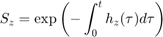
The hazard rate is integrated over time to yield the survival probability:
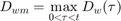
The IT model first finds the maximum of the scaled damage over time:
And then uses the cumulative distribution of the thresholds to find the survival probability:

This script: Long acute toxicity test for guppy (Poecilia reticulata) exposed to the insecticide dieldrin. Data from: Bedaux and Kooijman (1994), http://dx.doi.org/10.1007/BF00469427. This script deals with the basics only; many options for post-calculations are provided in the byom_guts_extra script.
Contents
Initial things
Make sure that this script is in a directory somewhere below the BYOM folder.
clear, clear global % clear the workspace and globals
global DATA W X0mat % make the data set and initial states global variables
global glo          % allow for global parameters in structure glo
global pri zvd      % global structures for optional priors and zero-variate data
diary off           % turn of the diary function (if it is accidentaly on)
% set(0,'DefaultFigureWindowStyle','docked'); % collect all figure into one window with tab controls
set(0,'DefaultFigureWindowStyle','normal'); % separate figure windows

pathdefine % set path to the BYOM/engine directory
glo.basenm  = mfilename; % remember the filename for THIS file for the plots
glo.saveplt = 0; % save all plots as (1) Matlab figures, (2) JPEG file or (3) PDF (see all_options.txt)
The data set
Data are entered in matrix form, time in rows, scenarios (exposure concentrations) in columns. First column are the exposure times, first row are the concentrations or scenario numbers. The number in the top left of the matrix indicates how to calculate the likelihood:
- -1 for multinomial likelihood (for survival data)
- 0 for log-transform the data, then normal likelihood
- 0.5 for square-root transform the data, then normal likelihood
- 1 for no transformation of the data, then normal likelihood
% observed number of survivors, time in days, conc. in ug/L
DATA{1} = [ -1  0  3.2  5.6  10  18  32  56  100
		0     20   20   20  20  20  20  20   20
		1     20   20   20  20  18  18  17    5
		2     20   20   19  17  15   9   6    0
		3     20   20   19  15   9   2   1    0
		4     20   20   19  14   4   1   0    0
		5     20   20   18  12   4   0   0    0
		6     20   19   18   9   3   0   0    0
		7     20   18   18   8   2   0   0    0 ];

% Note: For survival data, the weights matrix W has a different meaning
% than for continuous data: it can be used to specify the number of animals
% that went missing or were removed during the experiment (enter the number
% of missing/removed animals at the time they were last seen alive in the
% test). By default, the weights matrix for survival data is filled with
% zeros.

% scaled damage, can have no observations
DATA{2} = 0;
Initial values for the state variables
Initial states, scenarios in columns, states in rows. First row are the 'names' of all scenarios.
X0mat(1,:) = DATA{1}(1,2:end); % scenarios (concentrations)
X0mat(2,:) = 1;                % initial survival probability
X0mat(3,:) = 0;                % initial scaled damage
Initial values for the model parameters
Model parameters are part of a 'structure' for easy reference.
% global parameters for GUTS purposes
glo.sel  = 1; % select death mechanism: 1) SD 2) IT 3) mixed
glo.locD = 2; % location of scaled damage in the state variable list
glo.locS = 1; % location of survival probability in the state variable list

% start values for SD
% syntax: par.name = [startvalue fit(0/1) minval maxval optional:log/normal scale (0/1)];
par.kd = [0.5  1 1e-3  100 0];   % dominant rate constant, d-1
par.mw = [5    1    0  1e6 1];   % median threshold for survival (ug/L)
par.hb = [0.01 1    0    1 1];   % background hazard rate (1/d)
par.bw = [0.05 1 1e-6  1e6 0];   % killing rate (L/ug/d) (SD only)
par.Fs = [3    1    1  100 1];   % fraction spread of threshold distribution (IT only)

% % start values for IT
% % syntax: par.name = [startvalue fit(0/1) minval maxval optional:log/normal scale (0/1)];
% par.kd    = [0.001 1 1e-3 100 0]; % dominant rate constant (d-1)
% par.mw    = [0.06  1    0 1e6 1]; % median threshold for survival (ug/L)
% par.hb    = [0.001 1    0   1 1]; % background hazard rate (1/d)
% par.bw    = [0.04  1 1e-6 1e6 0]; % killing rate (L/ug/d) (SD and mixed)
% par.Fs    = [3.8   1    1 100 1]; % fraction spread of NEC distribution (-) (IT and mixed)

switch glo.sel % make sure that right parameters are fitted
    case 1 % for SD ...
        par.Fs(2) = 0; % never fit the threshold spread!
    case 2 % for IT ...
        par.bw(2) = 0; % never fit the killing rate!
    case 3 % mixed
        % do nothing: fit all parameters
end
Time vector and labels for plots
Specify what to plot. If time vector glo.t is not specified, a default is used, based on the data set
% specify the y-axis labels for each state variable
glo.ylab{1} = 'survival probability';
glo.ylab{2} = ['scaled damage (',char(181),'g/L)'];
% specify the x-axis label (same for all states)
glo.xlab    = 'time (days)';
glo.leglab1 = 'conc. '; % legend label before the 'scenario' number
glo.leglab2 = [char(181),'g/L']; % legend label after the 'scenario' number

prelim_checks % script to perform some preliminary checks and set things up
% Note: prelim_checks also fills all the options (opt_...) with defauls, so
% modify options after this call, if needed.
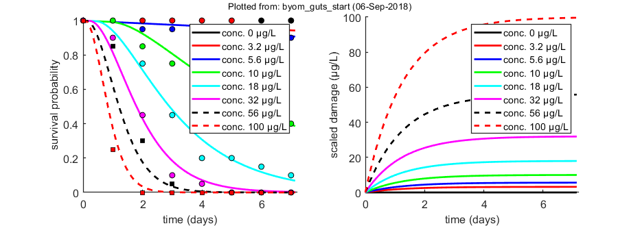
Calculations and plotting
Here, the function is called that will do the calculation and the plotting. Options for the plotting can be set using opt_plot (see prelim_checks.m). Options for the optimsation routine can be set using opt_optim. Options for the ODE solver are part of the global glo.
For the demo, the iterations were turned off (opt_optim.it = 0). In this case, the default position of the legend is obscuring part of the data and model lines. In byom_guts_extra.m an option is demonstrated to place the legend in a separate subplot.
glo.useode = 0; % calculate model using ODE solver (1) or analytical solution (0)
if glo.sel == 1 % for the pure SD model, turn on the events function to catch threshold exceedance
    glo.eventson = 1; % events function on (1) or off (0)
    % note: this is only used when glo.useode=1.
end

% par = start_vals_guts(par); % experimental start-value finder; use at your own risk
% % Note: start_vals will now overwrite the parameter structure par!

opt_optim.fit = 1; % fit the parameters (1), or don't (0)
opt_optim.it  = 0; % show iterations of the optimisation (1, default) or not (0)

% optimise and plot (fitted parameters in par_out)
par_out = calc_optim(par,opt_optim); % start the optimisation
calc_and_plot(par_out,opt_plot); % calculate model lines and plot them

% plot_guts(par_out,[],opt_guts); % uncomment to make more detailed plots
Goodness-of-fit measures for each data set (R-square)
    0.9869

Warning: R-square is not appropriate for survival data and needs to be
interpreted more qualitatively!

=================================================================================
Results of the parameter estimation with BYOM version 4.2b
=================================================================================
   Filename      : byom_guts_start
   Analysis date : 06-Sep-2018 (12:26)
   Data entered  :
     data state 1: 8x8, survival data.
     data state 2: 0x0, no data.
   Search method: Nelder-Mead simplex direct search, 2 rounds.
     The optimisation routine has converged to a solution
     Total 146 simplex iterations used to optimise.
     Minus log-likelihood has reached the value 161.527 (AIC=331.053).
=================================================================================
kd          0.791 (fit: 1, initial: 0.5)
mw          5.205 (fit: 1, initial:  5)
hb       0.008353 (fit: 1, initial: 0.01)
bw        0.03761 (fit: 1, initial: 0.05)
Fs              3 (fit: 0, initial:  3)
=================================================================================
Parameters kd and bw are fitted on log-scale.
=================================================================================
Time required: 0.7 secs
Plots result from the optimised parameter values.
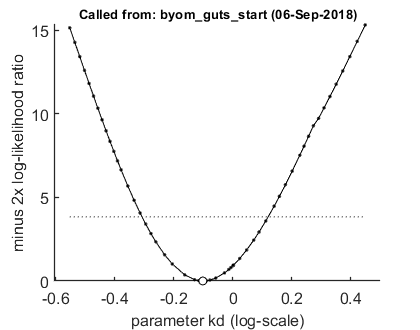
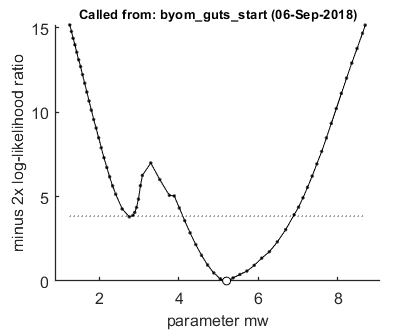
Profiling the likelihood
By profiling you make robust confidence intervals for one or more of your parameters. Use the name of the parameter as it occurs in your parameter structure par above. You do not need to run the entire script before you can make a profile.
Options for the profiling can be set using opt_prof (see prelim_checks). For this demo, no sub-optimisations are used. However, consider this options when working on your own data (e.g., set opt_prof.subopt=10).
The level of detail of the profiling is set to 'detailed' for this demo to catch the local optimum (it is just within the 95% CI, which is thus a broken set)
opt_prof.detail   = 1; % detailed (1) or a coarse (2) calculation
opt_prof.subopt   = 0; % number of sub-optimisations to perform to increase robustness

% UNCOMMENT FOLLOWING LINE(S) TO CALCULATE
% run a profile for selected parameters ...
calc_proflik(par_out,'kd',opt_prof);  % calculate a profile
calc_proflik(par_out,'mw',opt_prof);  % calculate a profile
95% confidence interval from the profile
=================================================================================
kd         interval:     0.4923 - 1.317

Time required: 13.4 secs

95% confidence interval from the profile
=================================================================================
The confidence interval is a broken set (check likelihood profile to check these figures)
mw         interval:
   interval 1:      2.742 - 2.8
   interval 2:      4.104 - 6.885

Time required: 19.3 secs
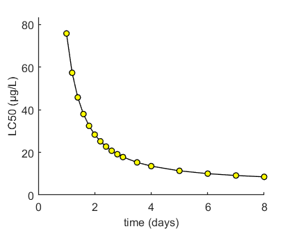
Calculate LCx versus time
Here, the LCx (by default the LC50) is calculated at several time points. When sufficient points are specified, a smooth line for LCx versus time will be produced. LCx values are also printed on screen. If a sample from parameter space is available (either from the slice sampler or the likelihood region), it can be used to calculate confidence bounds.
Options for LCx (with confidence bounds) can be set using opt_lcx (see prelim_checks).
% UNCOMMENT FOLLOWING LINE(S) TO CALCULATE
opt_conf.type = 0; % use the values from the slice sampler (1) or likelihood region (2) to make intervals (zero to skip)
Tend = [1:0.2:3 3.5 4:8]; % times at which to calculate LCx, relative to control

calc_conf_lcx_lim(par_out,Tend,opt_conf,opt_lcx); % calculates LCx values, CI requires that there is a mat file with sample
Calculate LCx values
Results table for LCx,t (µg/L)
==================================================================
LC50 (   1 days): 75.74
LC50 ( 1.2 days): 57.32
LC50 ( 1.4 days): 45.76
LC50 ( 1.6 days): 37.96
LC50 ( 1.8 days): 32.42
LC50 (   2 days): 28.32
LC50 ( 2.2 days): 25.18
LC50 ( 2.4 days): 22.71
LC50 ( 2.6 days): 20.74
LC50 ( 2.8 days): 19.13
LC50 (   3 days): 17.79
LC50 ( 3.5 days): 15.28
LC50 (   4 days): 13.55
LC50 (   5 days): 11.34
LC50 (   6 days): 10.01
LC50 (   7 days): 9.141
LC50 (   8 days): 8.526
==================================================================
No confidence intervals calculated
Other files: derivatives
To archive analyses, publishing them with Matlab is convenient. To keep track of what was done, the file derivatives.m can be included in the published result.
%% BYOM function derivatives.m (the model in ODEs)
%
%  Syntax: dX = derivatives(t,X,par,c)
%
% This function calculates the derivatives for the reduced GUTS model
% system. Note that the survival probability due to chemical stress is all
% calculated in <call_deri.html call_deri.m>. As input, it gets:
%
% * _t_   is the time point, provided by the ODE solver
% * _X_   is a vector with the previous value of the states
% * _par_ is the parameter structure
% * _c_   is the external concentration (or scenario number)
%
% Time _t_ and scenario name _c_ are handed over as single numbers by
% <call_deri.html call_deri.m> (you do not have to use them in this
% function). Output _dX_ (as vector) provides the differentials for each
% state at _t_.
%
% * Author: Tjalling Jager
% * Date: September 2018
% * Web support: <http://www.debtox.info/byom.html>
% * Back to index <walkthrough_guts.html>

%% Start

function dX = derivatives(t,X,par,c)

global glo          % allow for global parameters in structure glo (handy for switches)

%% Unpack states
% The state variables enter this function in the vector _X_. Here, we give
% them a more handy name.

S  = X(1); % state 1 is the survival probability at previous time point
Dw = X(2); % state 2 is the scaled damage at previous time point

%% Unpack parameters
% The parameters enter this function in the structure _par_. The names in
% the structure are the same as those defined in the byom script file.
% The 1 between parentheses is needed as each parameter has 5 associated
% values.

kd   = par.kd(1);   % dominant rate constant
% mw   = par.mw(1);   % median of threshold distribution (used in call_deri)
% bw   = par.bw(1);   % killing rate (used in call_deri)
% Fs   = par.Fs(1);   % fraction spread of threshold distribution, (-) (used in call_deri)
hb   = par.hb(1);   % background hazard rate

%% Extract correct exposure for THIS time point
% Allow for external concentrations to change over time, either
% continuously, or in steps, or as a static renewal with first-order
% disappearance. For constant exposure, the code in this section is skipped
% (and could also be removed).

if isfield(glo,'int_scen') % if it exists: use it to derive current external conc.
    if ismember(c,glo.int_scen) % is c in the scenario range global?
        c = make_scen(-1,c,t); % use make_scen again to derive actual exposure concentration
        % the -1 lets make_scen know we are calling from derivatives (so need one c)
    end
end

%% Calculate the derivatives
% This is the actual model, specified as a system of ODEs.

dDw = kd * (c - Dw); % first order damage build-up from c (scaled)
dS  = -hb* S; % only background hazard rate
% mortality due to the chemical is included in call_deri!

dX = [dS;dDw]; % collect derivatives in one vector
Other files: call_deri
To archive analyses, publishing them with Matlab is convenient. To keep track of what was done, the file call_deri.m can be included in the published result.
%% BYOM function call_deri.m (calculates the model output)
%
%  Syntax: [Xout TE] = call_deri(t,par,X0v)
%
% This function calls the ODE solver to solve the system of differential
% equations specified in <derivatives.html derivatives.m>, or the explicit
% function(s) in <simplefun.html simplefun.m>. As input, it gets:
%
% * _t_   the time vector
% * _par_ the parameter structure
% * _X0v_   a vector with initial states and one concentration (scenario number)
%
% The output _Xout_ provides a matrix with time in rows, and states in
% columns. This function calls <derivatives.html derivatives.m> or
% <simplefun.html simplefun.m>. The optional output _TE_ is the time at
% which an event takes place (specified using the events function). The
% events function is set up to catch discontinuities. It should be
% specified according to the problem you are simulating. If you want to use
% parameters that are (or influence) initial states, they have to be
% included in this function.
%
% This function is for the reduced GUTS model. The external function
% derivatives or simplefun provides the scaled damage over time and the
% background mortality. Mortality due to chemical stress is calculated in
% this function as a form of 'output mapping'.
%
% * Author: Tjalling Jager
% * Date: September 2018
% * Web support: <http://www.debtox.info/byom.html>
% * Back to index <walkthrough_guts.html>

%% Start

function [Xout,TE] = call_deri(t,par,X0v)

global glo   % allow for global parameters in structure glo
global zvd   % global structure for zero-variate data

%% Initial settings
% This part extracts optional settings for the ODE solver that can be set
% in the main script (defaults are set in prelim_checks). The useode option
% decides whether to calculate the model results using the ODEs in
% <derivatives.html derivatives.m>, or the analytical solution in
% <simplefun.html simplefun.m>. Using _eventson=1_ turns on the events
% handling. Also modify the sub-function at the bottom of this function!
% Further in this section, initial values can be determined by a parameter
% (overwrite parts of _X0_), and zero-variate data can be calculated. See
% the example BYOM files for more information.

useode   = glo.useode;   % calculate model using ODE solver (1) or analytical solution (0)
eventson = glo.eventson; % events function on (1) or off (0)
stiff    = glo.stiff;    % set to 1 or 2 to use a stiff solver instead of the standard one
min_t    = 500;          % minimum length of time vector (affects ODE stepsize as well)

% Unpack the vector X0v, which is X0mat for one scenario
X0 = X0v(2:end); % these are the intitial states for a scenario

%% Calculations
% This part calls the ODE solver (or the explicit model in <simplefun.html
% simplefun.m>) to calculate the output (the value of the state variables
% over time). There is generally no need to modify this part. The solver
% ode45 generally works well. For stiff problems, the solver might become
% very slow; you can try ode113 or ode15s instead.

c       = X0v(1); % the concentration (or scenario number)
t       = t(:);   % force t to be a row vector (needed when useode=0)
t_rem   = t;      % remember the original time vector (as we will add to it)

options = odeset; % start with default options for the ODE solver
% options = odeset(options, 'RelTol',1e-5,'AbsTol',1e-8); % specify tightened tolerances

if isfield(glo,'int_scen') && ismember(c,glo.int_scen) % is c in the scenario range global?
    % then we have a time-varying concentration
    Tev = make_scen(-2,c,-1); % use make_scen again to derive actual exposure concentration
    % the -2 lets make_scen know we need events, the -1 that this is also needed for splines!
    min_t = max(min_t,length(Tev(Tev(:,1)<t(end),1))*2);
    % For very long exposure profiles (e.g., FOCUS profiles), we now
    % automatically generate a larger time vector (twice the number of the
    % relevant points in the scenario).
    options = odeset(options,'InitialStep',t_rem(end)/(10*min_t),'MaxStep',t_rem(end)/min_t);
    % For the ODE solver, when we have a time-varying exposure set here, we
    % base minimum step size on min_t. Small stepsize is a good idea for
    % pulsed exposures; otherwise, stepsize may become so large that a
    % concentration change is missed completely.
else
    % options = odeset(options,'InitialStep',max(t)/100,'MaxStep',max(t)/10); % specify smaller stepsize
    % for constant concentrations, we can use a default or we can remove this option alltogether!
    % Matlab uses as default the length of the time vector divided by 10.
end
% For the GUTS cases, we need a long time vector. For the hazard and proper
% model, we need to numerically integrate the hazard rate over time. For IT
% in reduced models, we could make shortcuts, but since we don't know how
% people may modify the models in derivatives or simplefun, it is better to
% be general here. If the time span of the data set or simulation is very
% long (and the number of points in Tev is not), consider increasing the
% size of min_t.
if length(t) < min_t % make sure there are at least min_t points
    t = unique([t;(linspace(t(1),t(end),min_t))']);
end

TE = 0; % dummy for time of events
if useode == 1 % use the ODE solver to calculate the solution
    if eventson == 0 % if no events function is used ...
        switch stiff
            case 0
                [~,Xout] = ode45(@derivatives,t,X0,options,par,c);
            case 1
                [~,Xout] = ode113(@derivatives,t,X0,options,par,c);
            case 2
                [~,Xout] = ode15s(@derivatives,t,X0,options,par,c);
        end
    else % with an events functions ... additional output arguments for events:
        % TE catches the time of an event, YE the states at the event, and IE the number of the event
        options = odeset(options, 'Events',@eventsfun); % add an events function
        switch stiff % note that YE and IE can be added as additional outputs
            case 0
                [~,Xout,TE,~,~] = ode45(@derivatives,t,X0,options,par,c);
            case 1
                [~,Xout,TE,~,~] = ode113(@derivatives,t,X0,options,par,c);
            case 2
                [~,Xout,TE,~,~] = ode15s(@derivatives,t,X0,options,par,c);
        end
    end
    Xout = max(0,Xout); % in extreme cases, states can become ever so slightly negative

else % alternatively, use an explicit function provided in simplefun!
    Xout = simplefun(t,X0,par,c);
end

if isempty(TE) || all(TE == 0) % if there is no event caught
    TE = +inf; % return infinity
end

%% Output mapping
% _Xout_ contains a row for each state variable. It can be mapped to the
% data. If you need to transform the model values to match the data, do it
% here.
%
% This set of files is geared towards the use of the analytical solution
% for the damage level in simplefun (although it can also be used with the
% ODEs in derivatives). Therefore, only the damage level and background
% survival is available at this point, and the survival due to the chemical
% is added for each death mechanism below.

mw   = par.mw(1);             % median of threshold distribution
bw   = par.bw(1);             % killing rate
Fs   = max(1+1e-6,par.Fs(1)); % fraction spread of the threshold distribution
beta = log(39)/log(Fs);       % shape parameter for logistic from Fs
S    = Xout(:,glo.locS);      % take background survival from the model
Dw   = Xout(:,glo.locD);      % take the correct state variable for scaled damage

switch glo.sel
    case 1 % stochastic death
        haz    = bw * max(0,Dw-mw);          % calculate hazard for each time point
        cumhaz = cumtrapz(t,haz);            % integrate the hazard rate numerically
        S      = S .* min(1,exp(-1*cumhaz)); % calculate survival probability, incl. background

    case 2 % individual tolerance, log-logistic distribution is used
        mw = max(mw,1e-100); % make sure that the threshold is not exactly zero ...
        % New method to make sure that Dw does not decrease over time (dead
        % animals dont become alive). This increases speed, especially when
        % there is very little decrease in Dw.
        maxDw = Dw; % copy the vector Dw to maxDw
        ind   = find([0;diff(maxDw)]<0,1,'first'); % first index to places where Dw has decreased
        while ~isempty(ind) % as long as there is a decrease somewhere ...
            maxDw(ind:end) = max(maxDw(ind:end),maxDw(ind-1)); % replace every later time with max of that and previous point
            ind = find([0;diff(maxDw)]<0,1,'first'); % any decrease left?
        end
        S = S .* (1 ./ (1+(maxDw/mw).^beta)); % survival probability
        % the survival due to the chemical is multiplied with the background survival

    case 3 % mixed model
        % This is a fast way for GUTS proper. Damage is calculated only
        % once, as it is the same for all individuals. Survival for
        % different NECs is calculated below.
        n          = 200; % number of slices from the threshold distribution
        Fs2        = 999^(1/beta); % fraction spread for 99.9% of the distribution
        z_range    = linspace(mw/(1.5*Fs2),mw*Fs2,n); % range of NECs to cover 99.9%
        prob_range = ((beta/mw)*(z_range/mw).^(beta-1)) ./ ((1+(z_range/mw).^beta).^2); % pdf for the log-logistic (Wikipedia)
        prob_range = prob_range / sum(prob_range); % normalise the densities to exactly one
        S1         = zeros(length(t),1); % initialise the survival probability over time with zeros
        for i = 1:n % run through the different thresholds
            haz    = bw * max(0,Dw-z_range(i));  % calculate hazard for each NEC
            cumhaz = cumtrapz(t,haz);            % integrate the hazard rate numerically
            surv   = min(1,exp(-1*cumhaz));      % calculate survival probability
            S1     = S1 + surv * prob_range(i);  % add to S1, weighted for this NECs prob density
        end
        S = S .* S1; % make sure to add background hazard
end

Xout(:,glo.locS) = S;           % replace correct state by newly calculated survival prob.
[~,loct] = ismember(t_rem,t);   % find where the requested time points are in the long Xout
Xout = Xout(loct,:);            % only keep the ones we asked for

%% Events function
% Modify this part of the code if _eventson_=1.
% This subfunction catches the 'events': in this case, it looks for the
% internal concentration where the threshold is exceeded (only when
% useode=1). This only makes sense for SD.
%
% Note that the eventsfun has the same inputs, in the same sequence, as
% <derivatives.html derivatives.m>.

function [value,isterminal,direction] = eventsfun(t,X,par,c)

global glo

mw      = par.mw(1); % threshold for effects
nevents = 1;         % number of events that we try to catch

value      = zeros(nevents,1); % initialise with zeros
value(1)   = X(glo.locD) - mw; % thing to follow is dose metric minus threshold
isterminal = zeros(nevents,1); % do NOT stop the solver at an event
direction  = zeros(nevents,1); % catch ALL zero crossing when function is increasing or decreasing