BYOM, simple-compound model: byom_debtox_daphnia.m

Table of contents

About
Initial things
The data set
Initial values for the state variables
Initial values for the model parameters
Time vector and labels for plots
Calculations and plotting
Profiling the likelihood
Calculate ECx for all endpoints
Population growth rate
Other files: derivatives
Other files: call_deri

About

Author : Tjalling Jager
Date : November 2021
Web support: http://www.debtox.info/byom.html
Back to index walkthrough_debtox2019.html

BYOM is a General framework for simulating model systems in terms of ordinary differential equations (ODEs). The model itself needs to be specified in derivatives.m, and call_deri.m may need to be modified to the particular problem as well. The files in the engine directory are needed for fitting and plotting. Results are shown on screen but also saved to a log file (results.out).

The model: simple DEBtox model for toxicants, based on DEBkiss and formulated in compound parameters. The model includes flexible modules for toxicokinetics/damage dynamics and toxic effects. The DEBkiss e-book (see http://www.debtox.info/book_debkiss.html) provides a partial description of the model; the publication of Jager in Ecological Modelling contains the full details: https://doi.org/10.1016/j.ecolmodel.2019.108904.

This script: The water flea Daphnia magna exposed to fluoranthene; data set from Jager et al (2010), http://dx.doi.org/10.1007/s10646-009-0417-z. Published as case study in Jager & Zimmer (2012). Simultaneous fit on growth, reproduction and survival. Parameter estimates differ slightly from the ones in Jager & Zimmer due to several model changes and choices in the analysis.

Copyright (c) 2012-2021, Tjalling Jager, all rights reserved.
This source code is licensed under the MIT-style license found in the
LICENSE.txt file in the root directory of BYOM.

Initial things

Make sure that this script is in a directory somewhere below the BYOM folder.

clear, clear global % clear the workspace and globals
global DATA W X0mat % make the data set and initial states global variables
global glo          % allow for global parameters in structure glo
diary off           % turn of the diary function (if it is accidentaly on)
% set(0,'DefaultFigureWindowStyle','docked'); % collect all figure into one window with tab controls
set(0,'DefaultFigureWindowStyle','normal'); % separate figure windows

pathdefine(1) % set path to the BYOM/engine directory (option 1 uses parallel toolbox)
glo.basenm  = mfilename; % remember the filename for THIS file for the plots
glo.saveplt = 0; % save all plots as (1) Matlab figures, (2) JPEG file or (3) PDF (see all_options.txt)

The data set

Data are entered in matrix form, time in rows, scenarios (exposure concentrations) in columns. First column are the exposure times, first row are the concentrations or scenario numbers. The number in the top left of the matrix indicates how to calculate the likelihood:

-1 for multinomial likelihood (for survival data)
0 for log-transform the data, then normal likelihood
0.5 for square-root transform the data, then normal likelihood
1 for no transformation of the data, then normal likelihood

% scaled damage
DATA{1} = [0]; % there are never data for this state

% body length (mm) on each observation time (d), concentrations in uM
DATA{2} = [1 0 0 0.213	0.426	0.853
    0	0.88	0.88	0.88	0.88	0.88
    2	1.38	1.34	1.4     1.44	1.32
    4	1.96	1.72	1.9     1.88	1.74
    6	2.28	2.38	2.14	2.14	2.08
    8	2.34	2.52	2.56	2.36	2.16
    10	2.64	2.56	2.46	2.46	2.48
    12	2.66	2.56	2.6     2.58	2.7
    14	2.68	2.7     2.76	2.78	2.8
    16	2.88	2.78	2.82	NaN     NaN
    18	2.94	2.84	2.92	3.08	2.9
    20	3.06	3.02	3.02	3.22	2.76
    21	3.26	3.04	3.06	3       2.84];

W{2} = 5 * ones(size(DATA{2})-1); % weights: 5 animals in each treatment

% cumulative reproduction (nr. offspring per mother) (mm) on each
% observation time (d), concentrations in uM
DATA{3} = [1 0 0 	0.213	0.426	0.853
    0	0	0	0	0	0
    2	0	0	0	0	0
    4	0	0	0	0	0
    6	0	0	0	0	0
    8	1.2     2.1     0       0       0
    10	6.5     7.7     10.0	0.8     1.7
    12	17.9	25.4	16.3	2.0     1.7
    14	31.8	29.5	33.3	6.4     1.7
    16	50.6	48.8	56.2	9.4     1.7
    18	61.3	62.5	62.5	13.8	1.7
    20	81.0	76.4	64.1	16.4	1.7
    21	81.0	76.4	64.1	16.4	1.7];

% weights: number of individuals alive
W{3} = [10	10	10	10	10
	10	10	10	10	10
	10	10	10	10	10
	10	10	10	10	10
	10	10	10	10	10
	10	10	10	10	9
	10	10	10	10	7
	10	10	10	10	5
	10	10	10	10	5
	10	9	10	10	3
	10	9	10	9	3
	10	8	10	9	2];

% % In the next part, I subtract 3 days from the time vector for the repro
% % data; reason is that the eggs are produced some 3 days before the
% % offspring are counted. After this shift, the time vector thus represents
% % egg formation, which is the relevant trait for DEB analysis.
% DATA{3}(2:end,1) = DATA{3}(2:end,1) - 3; % extract x days from time vector
% DATA{3}([2 3],:) = []; % remove first two time points from DATA (t<0)
% W{3}([1 2],:)    = []; % remove first two time points from W (t<0)
% % This is not used here, instead glo.Tbp is used to shift model output by
% % three days.
glo.Tbp = 3; % shift model output for brood-pouch delay (rather than change the data set)

% survivors on each observation time (d), concentrations in uM
DATA{4} = [-1	0	0	0.213	0.426	0.853
    0	10	10	10	10	10
    2	10	10	10	10	10
    4	10	10	10	10	10
    6	10	10	10	10	10
    8	10	10	10	10	10
    10	10	10	10	10	9
    12	10	10	10	10	7
    14	10	10	10	10	5
    16	10	10	10	10	5
    18	10	9	10	10	3
    20	10	9	10	9	3
    21	10	8	10	9	2];

% if weight factors are not specified, ones are assumed in start_calc.m

Initial values for the state variables

Initial states, scenarios in columns, states in rows. First row are the 'names' of all scenarios.

X0mat = [0 0.213 0.426 0.853]; % the scenarios (here nominal concentrations)
X0mat(2,:) = 0; % initial values state 1 (scaled damage)
X0mat(3,:) = 0; % initial values state 2 (body length, initial value overwritten by L0)
X0mat(4,:) = 0; % initial values state 3 (cumulative reproduction)
X0mat(5,:) = 1; % initial values state 4 (survival probability)

% Put the position of the various states in globals, to make sure that the
% correct one is selected for extra things (e.g., for plotting in
% plot_tktd, in call_deri for accommodating 'no shrinking', for population
% growth rate).
glo.locD = 1; % location of scaled damage in the state variable list
glo.locL = 2; % location of body size in the state variable list
glo.locR = 3; % location of cumulative reproduction in the state variable list
glo.locS = 4; % location of survival probability in the state variable list

Initial values for the model parameters

Model parameters are part of a 'structure' for easy reference.

% global parameters as part of the structure glo
glo.FBV = 0.02;    % dry weight of egg as fraction of structural body weight (-) (for losses with reproduction)
glo.KRV = 1;       % part. coeff. repro buffer and structure (kg/kg) (for losses with reproduction)
glo.kap = 0.8;     % approximation for kappa (for starvation response)
glo.yP  = 0.8*0.8; % product of yVA and yAV (for starvation response)
glo.len = 2;       % set switch to 2 to prevent shrinking in length (used in call_deri.m)

% select mode of action of toxicant as set of switches:
% [assimilation/feeding, maintenance costs (somatic and maturity), growth costs, repro costs]
% glo.moa = [1 0 0 0 0]; % assimilation/feeding
% glo.moa = [0 1 0 0 0]; % costs for maintenance
% glo.moa = [0 0 1 1 0]; % costs for growth and reproduction
glo.moa = [0 0 0 1 0]; % costs for reproduction
% glo.moa = [0 0 0 0 1]; % hazards for reproduction

% select which feedbacks to use on damage dynamics as set of switches:
% [surface:volume on uptake, surface:volume on elimination, growth dilution, losses with reproduction]
% glo.feedb = [1 1 1 1]; % all feedbacks
glo.feedb = [1 1 1 0]; % classic DEBtox (no losses with repro)
% glo.feedb = [0 0 1 0]; % damage that is diluted by growth
% glo.feedb = [0 0 0 0]; % damage that is not diluted by growth

% syntax: par.name = [startvalue fit(0/1) minval maxval optional:log/normal scale (0/1)];
par.L0   = [1     1 0 1e6 1]; % body length at start experiment (mm)
par.Lp   = [1.8   1 0 1e6 1]; % body length at puberty (mm)
par.Lm   = [3     1 0 1e6 1]; % maximum body length (mm)
par.rB   = [0.15  1 0 1e6 1]; % von Bertalanffy growth rate constant (1/d)
par.Rm   = [10    1 0 1e6 1]; % maximum reproduction rate (#/d)
par.f    = [1     0 0   2 1]; % scaled functional response
par.hb   = [0.005 1 1e-6 1e6 0]; % background hazard rate (d-1)
% Note: it does not matter whether length measures are entered as actual
% length or as volumetric length (as long as the same measure is used
% consistently, and the organism is isomorphic).
% Note: hb is fitted on log-scale. This is especially helpful when hb is
% fitted along with the other parameters. The simplex fitting sometimes has
% trouble when one parameter is much smaller than others.

% extra parameters for special situations
par.Lf   = [0 0 0 1e6 1]; % body length at half-saturation feeding (mm)
par.Lj   = [0 0 0 1e6 1];  % body length at end acceleration (mm)
par.Tlag = [0 0 0  30 1]; % lag time for start development

ind_tox = length(fieldnames(par))+1; % index where tox parameters start

% the parameters below this line are all treated as toxicity parameters!
par.kd   = [0.076  1 0.01  10 0]; % dominant rate constant (d-1)
par.zb   = [0.096  1 0    1e6 1]; % effect threshold energy budget ([C])
par.bb   = [74     1 1e-6 1e6 0]; % effect strength energy-budget effect (1/[C])
par.zs   = [0.23   1 0    1e6 1]; % effect threshold survival ([C])
par.bs   = [0.66   1 1e-6 1e6 0]; % effect strength survival (1/([C] d))

Time vector and labels for plots

Specify what to plot. If time vector glo.t is not specified, a default is constructed, based on the data set.

% specify the y-axis labels for each state variable
glo.ylab{1} = ['scaled damage (',char(181),'M)'];
glo.ylab{2} = 'body length (mm)';
if isfield(glo,'Tbp') && glo.Tbp > 0
    glo.ylab{3} = ['cumul. repro. (shift ',num2str(glo.Tbp),'d)'];
else
    glo.ylab{3} = 'cumul. repro. (no shift)';
end
glo.ylab{4} = 'survival fraction (-)';

% specify the x-axis label (same for all states)
glo.xlab    = 'time (days)';
glo.leglab1 = 'conc. '; % legend label before the 'scenario' number
glo.leglab2 = [char(181),'M']; % legend label after the 'scenario' number

prelim_checks % script to perform some preliminary checks and set things up
% Note: prelim_checks also fills all the options (opt_...) with defauls, so
% modify options after this call, if needed.

Calculations and plotting

Here, the function is called that will do the calculation and the plotting. Options for the plotting can be set using opt_plot (see prelim_checks.m). Options for the optimsation routine can be set using opt_optim. Options for the ODE solver are part of the global glo.

NOTE: for this package, the options useode and eventson in glo will not be functional: the ODE solver is always used, and the events function as well.

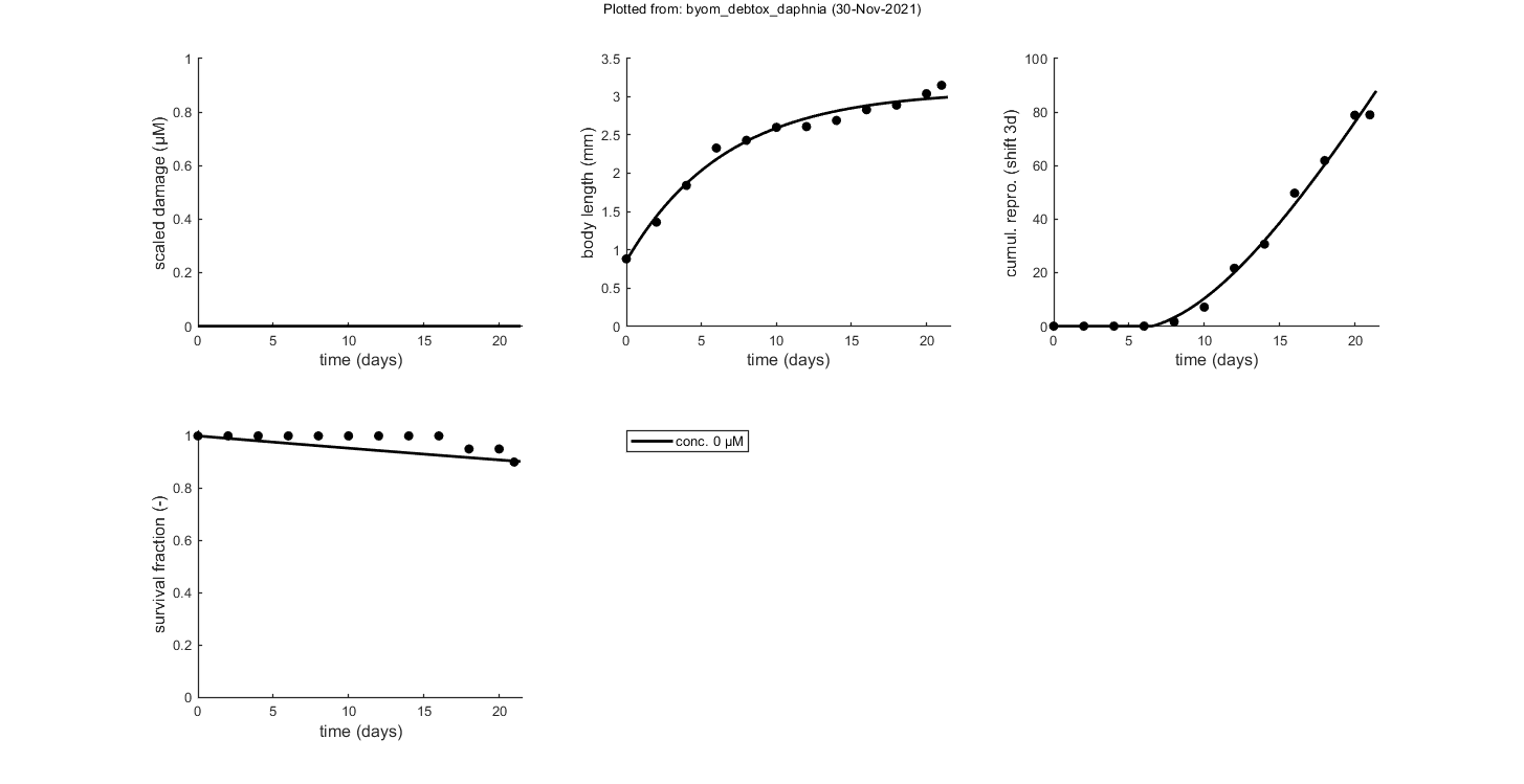
glo.stiff = [0 3]; % ODE solver 0) ode45 (standard), 1) ode113 (moderately stiff), 2) ode15s (stiff)
% Second argument is for normally tight (1), tighter (2), or very tight (3)
% tolerances. Use 1 for quick analyses, but check with 3 to see if there is
% a difference! Especially for time-varying exposure, there can be large
% differences between the settings!
glo.break_time = 0; % break time vector up for ODE solver (1) or don't (0)
% Note: breaking the time vector is a good idea when the exposure scenario
% contains discontinuities. Don't use for continuous splines (type 1) as it
% will be much slower. For FOCUS scenarios (high time resolution), breaking
% up is not efficient and does not appear to be necessary.

opt_optim.fit    = 1; % fit the parameters (1), or don't (0)
opt_optim.it     = 0; % show iterations of the optimisation (1, default) or not (0)
opt_plot.bw      = 0; % if set to 1, plots in black and white with different plot symbols
opt_plot.annot   = 2; % annotations in multiplot for fits: 1) box with parameter estimates 2) single legend
opt_plot.repls   = 0; % set to 1 to plot replicates, 0 to plot mean responses

% Note: using opt_optim.type = 4 (parspace explorer) would be served by
% setting a few more options. These settings can be ignored for other
% optimisation routines, but skip_sg must be defined before running
% automatic_runs.
opt_optim.ps_saved = 0; % use saved set for parameter-space explorer (1) or not (0);
opt_optim.ps_plots = 0; % when set to 1, makes intermediate plots of parameter space to monitor progress
opt_optim.ps_profs = 0; % when set to 1, makes profiles and additional sampling for parameter-space explorer
opt_optim.ps_rough = 1; % set to 1 for rough settings of parameter-space explorer, 0 for settings as in openGUTS
skip_sg            = 0; % set to 1 to skip startgrid completely (use ranges in <par> structure)

% The switch fit_tox is used to select whether to fit the control treatment
% (0), the toxicity treatments (1; the control is shown as well), or both
% together (2). A good strategy is to fit the basic parameters to the
% control data first (fit_tox=0), copy the best values into the parameter
% matrix above, and then fit the toxicity parameter to the complete data
% set (fit_tox=1). The code below automatically does that.

% ===== FITTING CONTROLS ==================================================
% Simplex fitting works fine for control data. Note that hb is fitted along
% with the other parameters.

opt_optim.type = 1; % optimisation method: 1) default simplex, 4) parspace explorer
fit_tox = [0]; % fit control parameters in data set
par_out = automatic_runs_basic(fit_tox,par,ind_tox,skip_sg,opt_optim,opt_plot);
% script to run the calculations and plot, automatically
par = copy_par(par,par_out,1); % copy fitted parameters into par, and keep fit mark in par

% ===== FITTING TOX DATA ==================================================
% Here, we can also use the parameter-space explorer for fitting the
% treatments. For the explorer, note that, with fit_tox=1, the tox
% parameters in par are replaced (when fitted) with estimates based on the
% data set using startgrid_debtox (called in automatic_runs). This is still
% quite experimental, so you may need to restart with manually-adapted
% ranges! Furthermore, this is really slow ... (the parallel toolbox really
% helps here!)
%
% For this demo, I use the regular simplex fitting. The parameter-space
% explorer is demonstrated for the ERA-special package

opt_optim.type = 1; % optimisation method 1) simplex, 4 parameter-space explorer
fit_tox = [1]; % fit tox parameters in data set
par_out = automatic_runs_basic(fit_tox,par,ind_tox,skip_sg,opt_optim,opt_plot);
disp_settings_debtox2019 % display some information on the settings on screen

% dedicated TKTD plots; these plots are more readable, especially when plotting CIs
opt_tktd.repls = 0; % plot individual replicates (1) or means (0)
if opt_optim.type == 4    % when the parspace explorer was used, we can plot with CIs ...
    opt_conf.type    = 3; % make intervals from parspace explorer
    opt_conf.lim_set = 2; % use limited set of n_lim points (1) or outer hull (2) to create CIs
    plot_tktd(par_out,opt_tktd,opt_conf);
else
    plot_tktd(par_out,opt_tktd,[]); % leave the options opt_conf empty to suppress all CIs for these plots
    % Note: plotting CIs requires a sample as saved by the various
    % methods available in BYOM (see examples directory).
end

% return % stops the analysis after optimisation/plotting; run the additional analyses below manually (or remove this line)

Goodness-of-fit measures for each state and each data set (R-square)
Based on the individual replicates, accounting for transformations, and including t=0
state 1.    NaN
state 2.   0.97
state 3.   0.99
state 4.  -0.34
Warning: R-square is not appropriate for survival data so interpret
qualitatively! 
Warning: (R-square not calculated when missing/removed animals; use plot_tktd) 
 
=================================================================================
Results of the parameter estimation with BYOM (par-engine) version 6.0 BETA 7
=================================================================================
   Filename      : byom_debtox_daphnia 
   Analysis date : 30-Nov-2021 (13:54) 
   Data entered  :
     data state 1: 0x0, no data.
     data state 2: 12x5, continuous data, no transf.
     data state 3: 12x5, continuous data, no transf.
     data state 4: 12x5, survival data.
   Search method: Nelder-Mead simplex direct search, 2 rounds. 
     The optimisation routine has converged to a solution
     Total 298 simplex iterations used to optimise. 
     Minus log-likelihood has reached the value 177.42 (AIC=366.84). 
=================================================================================
L0         0.8537 (fit: 1, initial:  1) 
Lp          1.782 (fit: 1, initial: 1.8) 
Lm          3.081 (fit: 1, initial:  3) 
rB         0.1513 (fit: 1, initial: 0.15) 
Rm          9.356 (fit: 1, initial: 10) 
f               1 (fit: 0, initial:  1) 
hb       0.004814 (fit: 1, initial: 0.005) 
Lf              0 (fit: 0, initial:  0) 
Lj              0 (fit: 0, initial:  0) 
Tlag            0 (fit: 0, initial:  0) 
kd          0.076 (fit: 0, initial: 0.076) 
zb          0.096 (fit: 0, initial: 0.096) 
bb             74 (fit: 0, initial: 74) 
zs           0.23 (fit: 0, initial: 0.23) 
bs           0.66 (fit: 0, initial: 0.66) 
=================================================================================
Parameter hb is fitted on log-scale.
=================================================================================
Mode of action used: 0  0  0  1  0
Feedbacks used     : 1  1  1  0
=================================================================================
Time required: 7.4 secs
Plots result from the optimised parameter values.

par.L0     = [    0.8537  1          0      1e+06 1]; 
par.Lp     = [    1.7825  1          0      1e+06 1]; 
par.Lm     = [    3.0813  1          0      1e+06 1]; 
par.rB     = [   0.15126  1          0      1e+06 1]; 
par.Rm     = [    9.3562  1          0      1e+06 1]; 
par.hb     = [ 0.0048136  1      1e-06      1e+06 0]; 
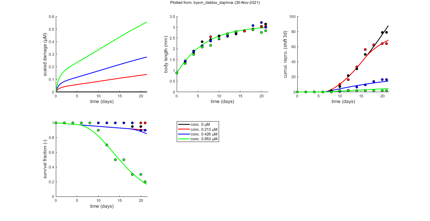
Goodness-of-fit measures for each state and each data set (R-square)
Based on the individual replicates, accounting for transformations, and including t=0
state 1.    NaN
state 2.   0.97
state 3.   0.99
state 4.   0.91
Warning: R-square is not appropriate for survival data so interpret
qualitatively! 
Warning: (R-square not calculated when missing/removed animals; use plot_tktd) 
 
=================================================================================
Results of the parameter estimation with BYOM (par-engine) version 6.0 BETA 7
=================================================================================
   Filename      : byom_debtox_daphnia 
   Analysis date : 30-Nov-2021 (13:54) 
   Data entered  :
     data state 1: 0x0, no data.
     data state 2: 12x5, continuous data, no transf.
     data state 3: 12x5, continuous data, no transf.
     data state 4: 12x5, survival data.
   Search method: Nelder-Mead simplex direct search, 2 rounds. 
     The optimisation routine has converged to a solution
     Total 119 simplex iterations used to optimise. 
     Minus log-likelihood has reached the value 498.20 (AIC=1006.40). 
=================================================================================
L0         0.8537 (fit: 0, initial: 0.8537) 
Lp          1.782 (fit: 0, initial: 1.782) 
Lm          3.081 (fit: 0, initial: 3.081) 
rB         0.1513 (fit: 0, initial: 0.1513) 
Rm          9.356 (fit: 0, initial: 9.356) 
f               1 (fit: 0, initial:  1) 
hb       0.004814 (fit: 0, initial: 0.004814) 
Lf              0 (fit: 0, initial:  0) 
Lj              0 (fit: 0, initial:  0) 
Tlag            0 (fit: 0, initial:  0) 
kd        0.07978 (fit: 1, initial: 0.076) 
zb        0.09881 (fit: 1, initial: 0.096) 
bb          71.63 (fit: 1, initial: 74) 
zs         0.2376 (fit: 1, initial: 0.23) 
bs         0.6410 (fit: 1, initial: 0.66) 
=================================================================================
Parameters kd, bb and bs are fitted on log-scale.
=================================================================================
Mode of action used: 0  0  0  1  0
Feedbacks used     : 1  1  1  0
=================================================================================
Time required: 28.0 secs
Plots result from the optimised parameter values.

 
========================================================================
Extra information on the model fit (DEBtox2019, stdDEB or extended GUTS)
Mode of action        : 0  0  0  1  0
Feedback configuration: 1  1  1  0
 
Model and ODE solver ----------------------------------------------
   Breaking time vector in call_deri: 0
   Settings for ODE solver call_deri: 0  3
   Brood-pouch delay for model (d)  : 3
Options for simplex optimisation-----------------------------------
   Number of sequential runs        : 2
===================================================================
 
Plot_tktd uses uses parameter set from user input for best-fit curves.
No confidence intervals are produced as opt_conf is empty

 
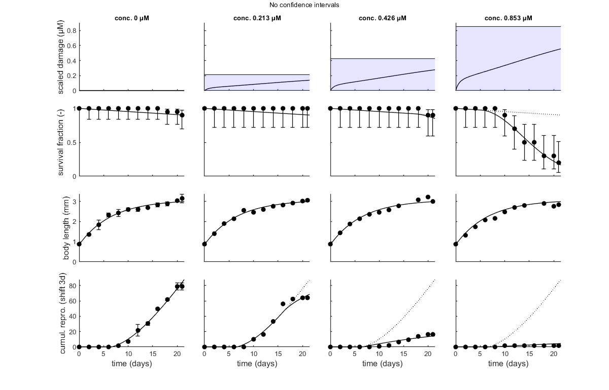
Goodness-of-fit metrics (treat with caution!)
 Values below are calculated on means, incl. t=0, from the residuals
 Residuals are used without accounting for any transformations
 However, means are calculated with transformation (if specified in DATA)
 
            Model efficiency (r2)   NRMSE
================================================================================
  survival    : 0.9371              0.0548 
  body length : 0.9767              0.0434 
  reproduction: 0.9878              0.1770 
================================================================================

Profiling the likelihood

By profiling you make robust confidence intervals for one or more of your parameters. Use the names of the parameters as they occurs in your parameter structure par above. This can be a single string (e.g., 'kd'), a cell array of strings (e.g., {'kd','mw'}), or 'all' to profile all fitted parameters. If you have used the parameter-space explorer for fitting, you already have (even more robust) profiles!

Options for the profiling can be set using opt_prof (see prelim_checks). For this demo, the level of detail of the profiling is set to 'coarse' and no sub-optimisations are used. However, consider these options when working on your own data (e.g., set opt_prof.subopt=10).

opt_prof.detail   = 2; % detailed (1) or a coarse (2) calculation
opt_prof.subopt   = 0; % number of sub-optimisations to perform to increase robustness
opt_prof.brkprof  = 2; % when a better optimum is located, stop (1) or automatically refit (2)

calc_proflik(par_out,'kd',opt_prof,opt_optim);  % calculate a profile
% Enter single parameter names, a cell array of names, or 'all' to profile
% all fitted parameters.

Starting parallel pool (parpool) using the 'local' profile ...
Connected to the parallel pool (number of workers: 8).

ans = 

 ProcessPool with properties: 

            Connected: true
           NumWorkers: 8
              Cluster: local
        AttachedFiles: {}
    AutoAddClientPath: true
          IdleTimeout: 30 minutes (30 minutes remaining)
          SpmdEnabled: true

Profiling is done using the parallel toolbox. No progress will be shown!

  
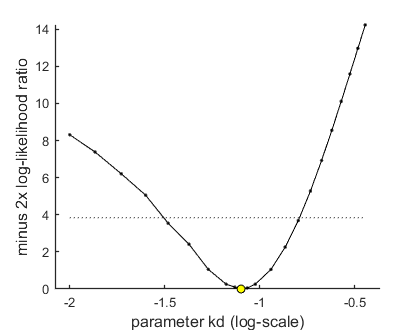
95% confidence interval(s) from the profile(s)
=================================================================================
kd         interval:    0.03123 -  0.1620 
=================================================================================
 
Time required: 2 mins, 14.6 secs

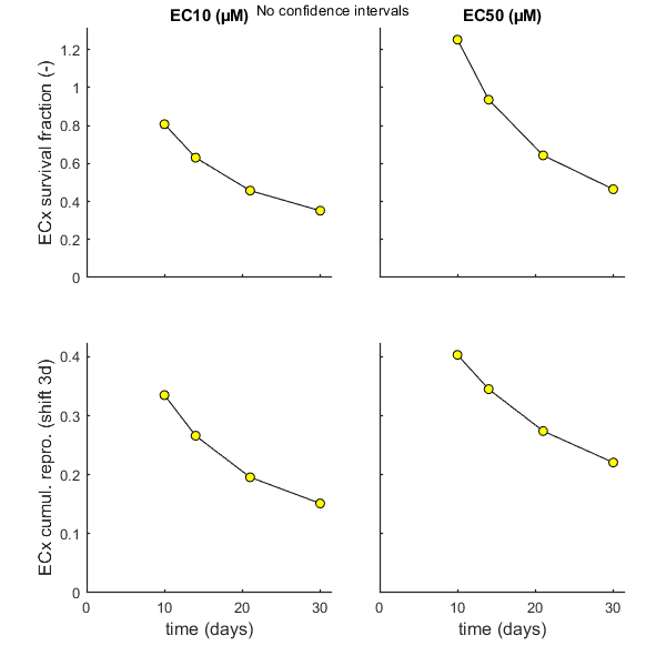
Calculate ECx for all endpoints

The function calc_ecx will calculate ECx values, based on the parameter values (and a sample from parameter space to make CIs). The ECx is calculated assuming constant exposure (which is in its definition) at the time points requested.

opt_conf.type    = 0; % make intervals from 1) slice sampler, 2)likelihood region, 3) parspace explorer
opt_conf.lim_set = 1; % use limited set of n_lim points (1) or outer hull (2, not for Bayes) to create CIs
opt_ecx.statsup  = []; % states to suppress from the calculations (e.g., glo.locS)

calc_ecx(par_out,[10 14 21 30],opt_ecx,opt_conf);
% Note that first input can be par_out, but if left empty it is read from
% the saved file (if it exists for the specified opt_conf.type). Second
% input is a vector with time points on which ECx is calculated (may extend
% beyond the time vector of the data set).

 
For body length, there is insufficient range of effects to calculate all ECx,t.
ECx without confidence intervals
================================================================================
time (days)    EC10 (95 perc. CI)    EC50 (95 perc. CI)    (µM)
================================================================================
  Survival    :
10.0      0.807 (       NaN -        NaN)       1.25 (       NaN -        NaN) 
14.0      0.631 (       NaN -        NaN)      0.936 (       NaN -        NaN) 
21.0      0.457 (       NaN -        NaN)      0.643 (       NaN -        NaN) 
30.0      0.352 (       NaN -        NaN)      0.465 (       NaN -        NaN) 
================================================================================
  Reproduction:
10.0      0.335 (       NaN -        NaN)      0.403 (       NaN -        NaN) 
14.0      0.266 (       NaN -        NaN)      0.345 (       NaN -        NaN) 
21.0      0.196 (       NaN -        NaN)      0.274 (       NaN -        NaN) 
30.0      0.151 (       NaN -        NaN)      0.221 (       NaN -        NaN) 
================================================================================
Boundaries used as min-max: 1e-07 - 1000000

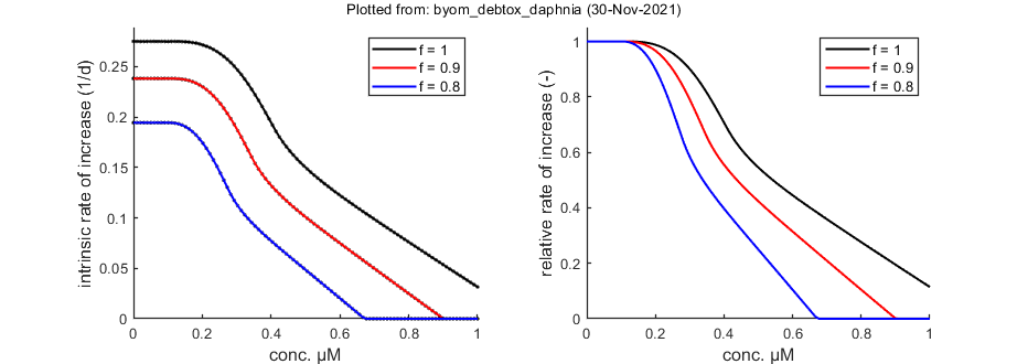
Population growth rate

The function calc_pop allows for a calculation of the intrinsic rate of population increase (Euler-Lotka equation). The function calc_pop needs checking ... so use with care! By default, the calculation is based on continuous reproduction (like the fit).

% Population calculations can be performed with CIs
opt_conf.type    = 0; % make intervals from 1) slice sampler, 2)likelihood region, 3) parspace explorer
opt_conf.lim_set = 0; % for lik-region sample: use limited set of n_lim points (1) or outer hull (2) to create CIs

Tpop = linspace(0,50,100); % time vector for the population calculations
Cpop = linspace(0,1,100); % concentration range for population calculations
% Cpop = -1; % use only concentrations as given in X0mat
Th = 3; % time from fresh egg to t=0 in time vector for experimental test (e.g., hatching time)
% Here, use 3 days, as this value was earlier subtracted from the time
% vector in the data set. So, reproduction now represents egg formation,
% and we need to account for hatching time in the population calculation.

calc_pop(par_out,X0mat,Tpop,Cpop,Th,opt_conf,opt_pop)

Other files: derivatives

To archive analyses, publishing them with Matlab is convenient. To keep track of what was done, the file derivatives.m can be included in the published result.

%% BYOM function derivatives.m (the model in ODEs)
%
%  Syntax: dX = derivatives(t,X,par,c,glo)
%
% This function calculates the derivatives for the model system. It is
% linked to the script files in the directory 'simple_compound'. As input,
% it gets:
% 
% * _t_   is the time point, provided by the ODE solver
% * _X_   is a vector with the previous value of the states
% * _par_ is the parameter structure
% * _c_   is the external concentration (or scenario number)
% * _glo_ is the structure with information (normally global)
%
% Time _t_ and scenario name _c_ are handed over as single numbers by
% <call_deri.html call_deri.m> (you do not have to use them in this
% function). Output _dX_ (as vector) provides the differentials for each
% state at _t_.
%
% * Author: Tjalling Jager
% * Date: November 2021
% * Web support: <http://www.debtox.info/byom.html>
% * Back to index <walkthrough_debtox2019.html>
% 
%  Copyright (c) 2012-2021, Tjalling Jager, all rights reserved.
%  This source code is licensed under the MIT-style license found in the
%  LICENSE.txt file in the root directory of BYOM. 

%% Start

function dX = derivatives(t,X,par,c,glo)

% NOTE: glo is now no longer a global here, but passed on in the function
% call from call_deri. That saves 20% calculation time!

%% Unpack states
% The state variables enter this function in the vector _X_. Here, we give
% them a more handy name.

X = max(X,0); % ensure the states cannot become negative due to numerical issues

Dw = X(1); % state is the scaled damage (referenced to water)
L  = X(2); % state is body length
% Rc = X(3); % state is cumulative reproduction (not used)
S  = X(4); % state is survival probability

%% Unpack parameters
% The parameters enter this function in the structure _par_. The names in
% the structure are the same as those defined in the byom script file.
% The 1 between parentheses is needed as each parameter has 5 associated
% values.

% unpack globals
FBV  = glo.FBV;     % dry weight of egg as fraction of dry body weight (-)
KRV  = glo.KRV;     % part. coeff. repro buffer and structure (kg/kg)
kap  = glo.kap;     % approximation for kappa (-)
yP   = glo.yP;      % product of yVA and yAV (-)

% unpack model parameters for the basic life history
L0   = par.L0(1);   % body length at start (mm)
Lp   = par.Lp(1);   % body length at puberty (mm)
Lm   = par.Lm(1);   % maximum body length (mm)
rB   = par.rB(1);   % von Bertalanffy growth rate constant (1/d)
Rm   = par.Rm(1);   % maximum reproduction rate (#/d)
f    = par.f(1);    % scaled functional response (-)
hb   = par.hb(1);   % background hazard rate (d-1)

% unpack extra parameters for specific cases
Lf   = par.Lf(1);   % body length at half-saturation feeding (mm)
Lj   = par.Lj(1);   % body length at which acceleration stops (mm)
Tlag = par.Tlag(1); % lag time for start development (d)

% unpack model parameters for the response to toxicants
kd   = par.kd(1);   % dominant rate constant (d-1)
zb   = par.zb(1);   % effect threshold energy budget ([C])
bb   = par.bb(1);   % effect strength energy-budget effects (1/[C])
zs   = par.zs(1);   % effect threshold survival ([C])
bs   = par.bs(1);   % effect strength survival (1/([C] d))

%% Extract correct exposure for THIS time point
% Allow for external concentrations to change over time, either
% continuously, or in steps, or as a static renewal with first-order
% disappearance. For constant exposure, the code in this section is skipped
% (and could also be removed). Note that glo.timevar is used to signal that
% there is a time-varying concentration. This option is set in call_deri.

if glo.timevar(1) == 1 % if we are warned that we have a time-varying concentration ...
    c = read_scen(-1,c,t,glo); % use read_scen to derive actual exposure concentration
    % Note: this has glo as input to the function to save time!
    % the -1 lets read_scen know we are calling from derivatives (so need one c)
end

%% Calculate the derivatives
% This is the actual model, specified as a system of ODEs. This is the
% DEBkiss model, with toxicant effects and starvation module, expressed in
% terms of compound parameters, as presented in the publication (Jager,
% 2020).

L = max(1e-3*L0,L); % make sure that body length is not negative or almost zero (extreme shrinking may do that)
% This should not be needed as shrinking is limited at the bottom of this
% function.

if Lf > 0 % to include feeding limitation for juveniles ...
    f  = f / (1+(Lf^3)/(L^3)); % hyperbolic relationship for f with body volume
    % kd = kd*f; % also reduce dominant rate by same factor? (open for discussion!)
end
if Lj > 0 % to include acceleration until metamorphosis ...
    f = f * min(1,L/Lj); % this implies lower f for L<Lj
end

% Calculate stress factor and hazard rate.
s = bb*max(0,Dw-zb); % stress level for metabolic effects
h = bs*max(0,Dw-zs); % hazard rate for effects on survival

% Define specific stress factors s*, depending on the mode of action as
% specified in the vector with switches glo.moa.
Si = glo.moa * s;  % vector with specific stress factors from switches for mode of action
sA = min(1,Si(1)); % assimilation/feeding (maximise to 1 to avoid negative values for 1-sA)
sM = Si(2);        % maintenance (somatic and maturity)
sG = Si(3);        % growth costs
sR = Si(4);        % reproduction costs               
sH = Si(5);        % also include hazard to reproduction

% Calcululate the actual derivatives, with stress implemented.
dL = rB * ((1+sM)/(1+sG)) * (f*Lm*((1-sA)/(1+sM)) - L); % ODE for body length

fR = f; % if there is no starvation, f for reproduction is the standard f
% starvation rules can modify the outputs here
if dL < 0 % then we are looking at starvation and need to correct things
    fR = (f - kap * (L/Lm) * ((1+sM)/(1-sA)))/(1-kap); % new f for reproduction alone
    if fR >= 0  % then we are in the first stage of starvation: 1-kappa branch can help pay maintenance
        dL = 0; % stop growth, but don't shrink
    else        % we are in stage 2 of starvation and need to shrink to pay maintenance
        fR = 0; % nothing left for reproduction
        dL = (rB*(1+sM)/yP) * ((f*Lm/kap)*((1-sA)/(1+sM)) - L); % shrinking rate
    end
end
        
R  = 0; % reproduction rate is zero, unless ... 
if L >= Lp % if we are above the length at puberty, reproduce
    R = max(0,(exp(-sH)*Rm/(1+sR)) * (fR*Lm*(L^2)*(1-sA) - (Lp^3)*(1+sM))/(Lm^3 - Lp^3));
end

dRc = R;             % cumulative reproduction rate
dS  = -(h + hb) * S; % change in survival probability (incl. background mort.)

% For the damage dynamics, there are four feedback factors x* that obtain a
% value based on the settings in the configuration vector glo.feedb: a
% vector with switches for various feedbacks: [surface:volume on uptake,
% surface:volume on elimination, growth dilution, losses with
% reproduction].
Xi = glo.feedb .* [Lm/L,Lm/L,(3/L)*dL,R*FBV*KRV]; % multiply switch factor with feedbacks
xu = Xi(1); % factor for surf:vol scaling uptake rate 
xe = Xi(2); % factor for surf:vol scaling elimination rate 
xG = Xi(3); % factor for growth dilution
xR = Xi(4); % factor for losses with repro

% if switch for surf:vol scaling is zero, the factor must be 1 and not 0!
% Note: this was previously done with a max-to-1 command. However, that is
% a bit dangerous when modifying the model.
if Xi(1) == 0
    xu = 1;
end
if Xi(2) == 0
    xe = 1;
end

xG = max(0,xG); 
% NOTE NOTE: reverse growth dilution (concentration by shrinking) is now
% turned OFF as it leads to runaway situations that lead to failure of the
% ODE solvers. However, this needs some further thought!

dDw = kd * (xu * c - xe * Dw) - (xG + xR) * Dw; % ODE for scaled damage

if L <= 0.5 * L0 % if an animal has size less than half the start size ...
    dL = 0; % don't let it grow or shrink any further (to avoid numerical issues)
end

dX = zeros(size(X)); % initialise with zeros in right format
if t >= Tlag % when we are past the lag time ...
    dX = [dDw;dL;dRc;dS]; % collect all derivatives in one vector dX
end

Other files: call_deri

To archive analyses, publishing them with Matlab is convenient. To keep track of what was done, the file call_deri.m can be included in the published result.

%% BYOM function call_deri.m (calculates the model output)
%
%  Syntax: [Xout,TE,Xout2,zvd] = call_deri(t,par,X0v,glo)
%
% This function calls the ODE solver to solve the system of differential
% equations specified in <derivatives.html derivatives.m>. It is specific
% for the model in the directory 'simple_compound', and modified to deal
% with time-varying exposure by splitting up the ODE solving to avoid hard
% switches. 
% 
% As input, it gets:
% * _t_   the time vector
% * _par_ the parameter structure
% * _X0v_   a vector with initial states and one concentration (scenario number)
% * _glo_ the structure with various types of information (used to be global)
%
% The output _Xout_ provides a matrix with time in rows, and states in
% columns. This function calls <derivatives.html derivatives.m>. The
% optional output _TE_ is the time at which an event takes place (specified
% using the events function). The events function is set up to catch
% discontinuities. It should be specified according to the problem you are
% simulating. If you want to use parameters that are (or influence) initial
% states, they have to be included in this function. Optional output Xout2
% is for additional uni-variate data (not used here), and zvd is for
% zero-variate data (not used here).
%
% * Author: Tjalling Jager
% * Date: November 2021
% * Web support: <http://www.debtox.info/byom.html>
% * Back to index <walkthrough_debtox2019.html>
% 
%  Copyright (c) 2012-2021, Tjalling Jager, all rights reserved.
%  This source code is licensed under the MIT-style license found in the
%  LICENSE.txt file in the root directory of BYOM. 

%% Start

function [Xout,TE,Xout2,zvd] = call_deri(t,par,X0v,glo)

% These outputs need to be defined, even if they are not used
Xout2    = []; % additional uni-variate output, not used in this example
zvd      = []; % additional zero-variate output, not used in this example

%% Initial settings
% This part extracts optional settings for the ODE solver that can be set
% in the main script (defaults are set in prelim_checks). Further in this
% section, initial values can be determined by a parameter (overwrite parts
% of X0), and zero-variate data can be calculated. See the example BYOM
% files for more information.
% 
% This package will always use the ODE solver; therefore the general
% settings in the global glo for the calculation (useode and eventson) are
% removed here. This packacge also always uses the events function, so the
% option eventson is not used. Furthermore, simplefun.m is removed.

stiff      = glo.stiff; % ODE solver 0) ode45 (standard), 1) ode113 (moderately stiff), 2) ode15s (stiff)
break_time = glo.break_time; % break time vector up for ODE solver (1) or don't (0)
min_t      = 500; % minimum length of time vector (affects ODE stepsize only, when needed)

if length(stiff) == 1
    stiff(2) = 1; % by default: normally tightened tolerances
end

% Unpack the vector X0v, which is X0mat for one scenario
X0 = X0v(2:end); % these are the intitial states for a scenario
c  = X0v(1); % the concentration (or scenario number)

% Start with a check on time-varying exposure scenarios. This is a
% time-saver! The isfield and ismember calls take some time that rapidly
% multiplies as derivatives is called many times.
glo.timevar = [0 0]; % flag for time-varying exposure (second element is to tell read_scen which interval we need)
if isfield(glo,'int_scen') && ismember(c,glo.int_scen) % is c in the scenario range of the global?
    glo.timevar = [1 0]; % tell derivatives that we have a time-varying treatment
end

% if needed, extract parameters from par that influence initial states in X0
% start from specified initial size in a model parameter
L0 = par.L0(1); % initial body length (mm) is a parameter
X0(glo.locL) = L0; % put this estimate in the correct location of the initial vector

%% Calculations
% This part calls the ODE solver to calculate the output (the value of the
% state variables over time). There is generally no need to modify this
% part. The solver ode45 generally works well. For stiff problems, the
% solver might become very slow; you can try ode15s instead.

t     = t(:);   % force t to be a row vector (needed when useode=0)
t_rem = t;      % remember the original time vector (as we will add to it)

% The code below is meant for discontinous time-varying exposure. It will
% also work for constant exposure. Breaking up will not be as effective for
% piecewise polynomials (type 1), and slow, so better turn that off
% manually when you try splining. The code will run each interval between
% two exposure 'events' (in Tev) separately, stop the solver, and restart.
% This ensures that the discontinuities are no problem anymore.

TE  = 0; % dummy for time of events in the events function
Tev = [0 c]; % exposure profile events setting: without anything else, assume it is constant

InitialStep = max(t)/100; % specify initial stepsize
MaxStep     = max(t)/10;  % specify maximum stepsize
% For constant concentrations, and when breaking the time vector, we can
% use a default; Matlab uses as default the length of the time vector
% divided by 10.

if glo.timevar(1) == 1 % time-varying concentrations?
    % if it exists: use it to derive time vector for the events in the exposure scenario    
    Tev = read_scen(-2,c,-1,glo); % use read_scen to derive exposure concentration events
    % the -2 lets read_scen know we need events, the -1 that this is also needed for splines!
    
    min_t = max(min_t,length(Tev(Tev(:,1)<t(end),1))*2); 
    % For very long exposure profiles (e.g., FOCUS profiles), we now
    % automatically generate a larger time vector (twice the number of the
    % relevant points in the scenario). This is only used to set step size
    % when not using break_time, and for locating maximum length under
    % no-shrinking.
    
    if break_time == 0
        InitialStep = t(end)/(10*min_t); % initial step size
        MaxStep     = t(end)/min_t;      % maximum step size
        % For the ODE solver, when we have a time-varying exposure set
        % here, we base minimum step size on min_t. Small stepsize is a
        % good idea for pulsed exposures; otherwise, stepsize may become so
        % large that a concentration change is missed completely. When we
        % break the time vector, limiting step size is not needed.
    end
end

% This is a means to include a delay caused by the brood pounch in species
% like Daphnia. The repro data are for the appearance of neonates, but egg
% production occurs earlier. This global shifts the model output in this
% function below. This way, the time vector in the data does not need to be
% manipulated, and the model plots show the neonate production as expected.
bp = 0; % by default, no brood-pouch delay
if isfield(glo,'Tbp') && glo.Tbp > 0 % if there is a global specifying a brood-pouch delay ...
    tbp = t(t>glo.Tbp)-glo.Tbp; % extra times needed to calculate brood-pounch delay
    t   = unique([t;tbp]);      % add the shifted time points to account for brood-pouch delay
    bp  = 1;                    % signal rest of code that we need brood-pouch delay
end

% When an animal cannot shrink in length, we need a long time vector as we
% need to catch the maximum length over time.
if glo.len == 2 && length(t) < min_t % make sure there are at least min_t points
    t = unique([t;(linspace(t(1),t(end),min_t))']);
end

% specify options for the ODE solver
options = odeset; % start with default options for the ODE solver
% This needs further study ... events function removed. Events function
% needs to be considered very carefully for this model (and would only be
% useful for SD).
switch stiff(2)
    case 1 % for ODE15s, slightly tighter tolerances seem to suffice (for ODE113: not tested yet!)
        RelTol  = 1e-4; % relative tolerance (tightened)
        AbsTol  = 1e-7; % absolute tolerance (tightened)
    case 2 % somewhat tighter tolerances ...
        RelTol  = 1e-5; % relative tolerance (tightened)
        AbsTol  = 1e-8; % absolute tolerance (tightened)
    case 3 % for ODE45, very tight tolerances seem to be necessary in some cases
        RelTol  = 1e-9; % relative tolerance (tightened)
        AbsTol  = 1e-9; % absolute tolerance (tightened)
end
options = odeset(options,'RelTol',RelTol,'AbsTol',AbsTol,'Events',@eventsfun,'InitialStep',InitialStep,'MaxStep',MaxStep); % set options
% Note: setting tolerances is pretty tricky. For some cases, tighter
% tolerances are needed but not for others. For ODE45, tighter tolerances
% seem to work well, but not for ODE15s.

T = Tev(:,1); % time vector with events
if T(end) > t(end) % scenario may be longer than t(end)
    T(T>t(end)) = []; % remove all entries that are beyond the last time point
    % this may remove one point too many, but that will be added next
end
if T(end) < t(end) % scenario may (now) be shorter than we need
    T = cat(1,T,t(end)); % then add last point from t
end
% If a lag time is used, it is a good idea to add it as an event as ODE45
% does not like such a switch either.
Tlag = par.Tlag(1);
if Tlag > 0
    T = unique([par.Tlag(1);T]);
end

% Breaking up the time vector is faster and more robust when calibrating on
% data from time-varying exposure that contain discontinuities. However,
% when running through very detailed exposure profiles (e.g., those from
% FOCUS), it is probably best to use break_time=0. Testing indicates that
% breaking up will be much slower than simply running the ODE solver across
% the entire profile (and produces very similar output).
% 
% Note: it is possible to initialise tout and Xout with NaNs, and avoid
% these matrices to grow. This may be a bit slower for exposure scenarios
% with few events, but faster for scenarios with many.

t = unique([T;t;(T(1:end-1)+T(2:end))/2]); % combine T, t, and halfway-T into new time vector
% this hopefully prevents the ODE solver from missing exposure pulses, and
% it makes sure that, for break_time=1, we never have a temporary time
% vector of length 2.

if break_time == 0 
    
    % simply use the ODE solver for the entire time vector    
    switch stiff(1)
        case 0
            [tout,Xout,TE,~,~] = ode45(@derivatives,t,X0,options,par,c,glo);
        case 1
            [tout,Xout,TE,~,~] = ode113(@derivatives,t,X0,options,par,c,glo);
        case 2
            [tout,Xout,TE,~,~] = ode15s(@derivatives,t,X0,options,par,c,glo);
    end
    
else
    
    % Transferring the interval to derivatives is a huge time saver! It is
    % not safe to use i as index to Tev since we may add Tlag to T (which
    % is not in Tev); so better calculate it explicitly. Using <find> may
    % be a bit slow, that is why this is done outside of the loop calling
    % the ODE solver.
    ind_Tev = zeros(length(T)-1,1);
    for i = 1:length(T)-1 % run through all intervals between events
        ind_Tev(i) = find(Tev(:,1) <= T(i),1,'last');
    end
    
    % NOTE: predefining *should* increase speed, but the speed gain is not
    % so clear in this case. I expect some gain when using many exposure
    % intervals.
    tout    = nan(length(t)+5,1); % this vector will collect the time output from the solver (5 more than needed)
    Xout    = nan(length(tout),length(X0)); % this matrix will collect the states output from the solver (5 more than needed)
    ind_i   = 1; % index for where we are in tout and Xout
    % Note: I initialise tout and Xout with more than the elements of t
    % because the events may be added as well (only stopping events, which
    % are not used yet). The number is rather arbitrary but should be equal
    % to, or more than, the number of events.

    % run the ODE solver piece-wise across all exposure events specified
    for i = 1:length(T)-1 % run through all intervals between events
        t_tmp = [T(i);T(i+1)]; % start with start and end time for this period
        t_tmp = unique([t_tmp;t(t<t_tmp(2) & t>t_tmp(1))]); % and add the time points from t that fit in there
        glo.timevar(2) = ind_Tev(i); % tell derivatives which part of Tev we're in
        
        % NOTE: adding a time point in between when t_tmp is length 2 is
        % not needed. We've added T and half-way-into T into time vector t.
        % Since we do NOT stop at events, there is no way to have a time
        % vector of two elements!

        % use ODE solver to find solution in this interval
        % Note: the switch-case may be compromising calculation speed; however,
        % it needs to be investigated which solver performs best
        switch stiff(1)
            case 0
                [tout_tmp,Xout_tmp,TE,~,~] = ode45(@derivatives,t_tmp,X0,options,par,c,glo);
            case 1
                [tout_tmp,Xout_tmp,TE,~,~] = ode113(@derivatives,t_tmp,X0,options,par,c,glo);
            case 2
                [tout_tmp,Xout_tmp,TE,~,~] = ode15s(@derivatives,t_tmp,X0,options,par,c,glo);
        end
        
        % collect output in correct location
        nt = length(tout_tmp); % length of the output time vector
        tout(ind_i:ind_i-1+nt)   = tout_tmp; % add tout_tmp to correct position in tout
        Xout(ind_i:ind_i-1+nt,:) = Xout_tmp; % add Xout_tmp to correct position in Xout

        ind_i = ind_i-1+nt;       % update ind_i for next round
        X0    = Xout_tmp(end,:)'; % update X0 for next round
        % Note: the way ind_i is used, there will be no double time points
        % in tout and Xout.
    end
    
end

if isempty(TE) || all(TE == 0) % if there is no event caught
    TE = +inf; % return infinity
end
% This is not so useful as only the TE found in the last time period is
% returned.

%% Output mapping
% _Xout_ contains a row for each state variable. It can be mapped to the
% data. If you need to transform the model values to match the data, do it
% here. 

if glo.len == 2 % when animal cannot shrink in length (but does on weight!)
    L     = Xout(:,glo.locL); % take correct state for body lenght
    maxL  = cummax(L); % copy the vector L to maxL and find cumulative maximum
    Xout(:,glo.locL) = maxL; % replace length is Xout with new maximised body length
end

Xout(:,glo.locS) = max(0,Xout(:,glo.locS)); % make sure survival does not get negative
% In some case, it may become just a bit negative, which means zero.

if bp == 1 % if we need a brood-pouch delay ... 
    [~,loct] = ismember(tbp,tout); % find where the extra brood-pouch time points are in the long Xout
    Xbp      = Xout(loct,glo.locR); % only keep the brood-pouch ones we asked for
end
t = t_rem; % return t to the original input vector

% Select the correct time points to return to the calling function
[~,loct] = ismember(t,tout); % find where the requested time points are in the long Xout
Xout     = Xout(loct,:);     % only keep the ones we asked for

if bp == 1 % if we need a brood-pouch delay ... 
    [~,loct] = ismember(tbp+glo.Tbp,t); % find where the extra brood-pouch time points SHOULD BE in the long Xout
    Xout(:,glo.locR)    = 0;   % clear the reproduction state variable
    Xout(loct,glo.locR) = Xbp; % put in the brood-pouch ones we asked for
end

% % To obtain the output of the derivatives at each time point. The values in
% % dXout might be used to replace values in Xout, if the data to be fitted
% % are the changes (rates) instead of the state variable itself.
% % dXout = zeros(size(Xout)); % initialise with zeros
% for i = 1:length(t) % run through all time points
%     dXout(i,:) = derivatives(t(i),Xout(i,:),par,c,glo); 
%     % derivatives for each stage at each time
% end

%% Events function
% This subfunction catches the 'events': in this case, this one catches
% when the scaled damage exceeds one of the thresholds, and catches the
% switch at puberty.
%
% Note that the eventsfun has the same inputs, in the same sequence, as
% <derivatives.html derivatives.m>.

function [value,isterminal,direction] = eventsfun(t,X,par,c,glo)

% Note: glo needs to be an input to the events function as well, rather
% than a global since the inputs for the events function must match those
% for derivatives.

Lp = par.Lp(1); % length at puberty (mm)
zb = par.zb(1); % effect threshold for the energy budget
zs = par.zs(1); % effect threshold for survival

nevents = 3; % number of events that we try to catch

value    = zeros(nevents,1); % initialise with zeros
value(1) = X(glo.locD) - zb; % follow when scaled damage exceeds the effect threshold for the energy budget
value(2) = X(glo.locD) - zs; % follow when scaled damage exceed the effect threshold for survival
value(3) = X(glo.locL) - Lp; % follow when body length exceeds length at puberty

isterminal = zeros(nevents,1); % do NOT stop the solver at an event
direction  = zeros(nevents,1); % catch ALL zero crossing when function is increasing or decreasing