BYOM, byom_debtox_daphnia_auto.m, DEBtox with Daphnia
- Author: Tjalling Jager
- Date: November 2021
- Web support: http://www.debtox.info/byom.html
- Back to index walkthrough_debtox.html
BYOM is a General framework for simulating model systems in terms of ordinary differential equations (ODEs). The model itself needs to be specified in derivatives.m, and call_deri.m may need to be modified to the particular problem as well. The files in the engine directory are needed for fitting and plotting. Results are shown on screen but also saved to a log file (results.out).
The model: DEBtox following Jager & Zimmer (2012), http://dx.doi.org/10.1016/j.ecolmodel.2011.11.012.
This script: The water flea Daphnia magna exposed to fluoranthene; data set from Jager et al (2010), http://dx.doi.org/10.1007/s10646-009-0417-z. Published as case study in Jager & Zimmer (2012). Simultaneous fit on growth, reproduction and survival. Parameter estimates differ slightly from the ones in Jager & Zimmer as we here take the two controls as seperate treatments (with the same parameters). This script demonstrates an automatic procedure to first fit the basic parameters to the controls, and next the tox parameters on the entire data set (fixing the basic parameters). It furthermore demonstrates the use of the parameter-space explorer for fitting the tox parameters.
Copyright (c) 2012-2021, Tjalling Jager, all rights reserved.
This source code is licensed under the MIT-style license found in the
LICENSE.txt file in the root directory of BYOM.
Contents
Initial things
Make sure that this script is in a directory somewhere below the BYOM folder.
clear, clear global % clear the workspace and globals
global DATA W X0mat % make the data set and initial states global variables
global glo          % allow for global parameters in structure glo
diary off           % turn of the diary function (if it is accidentaly on)
% set(0,'DefaultFigureWindowStyle','docked'); % collect all figure into one window with tab controls
set(0,'DefaultFigureWindowStyle','normal'); % separate figure windows

pathdefine(1) % set path to the BYOM/engine directory (1 uses parallel toolbox, when available)
glo.basenm  = mfilename; % remember the filename for THIS file for the plots
glo.saveplt = 0; % save all plots as (1) Matlab figures, (2) JPEG file or (3) PDF (see all_options.txt)
The data set
Data are entered in matrix form, time in rows, scenarios (exposure concentrations) in columns. First column are the exposure times, first row are the concentrations or scenario numbers. The number in the top left of the matrix indicates how to calculate the likelihood:
- -1 for multinomial likelihood (for survival data)
- 0 for log-transform the data, then normal likelihood
- 0.5 for square-root transform the data, then normal likelihood
- 1 for no transformation of the data, then normal likelihood
% scaled damage
DATA{1} = [0]; % there are never data for this state

% scaled reserve density
DATA{2} = [0]; % there are never data for this state

% body length (mm) on each observation time (d), concentrations in uM
DATA{3} = [1 0 0 0.213	0.426	0.853
    0	0.88	0.88	0.88	0.88	0.88
    2	1.38	1.34	1.4     1.44	1.32
    4	1.96	1.72	1.9     1.88	1.74
    6	2.28	2.38	2.14	2.14	2.08
    8	2.34	2.52	2.56	2.36	2.16
    10	2.64	2.56	2.46	2.46	2.48
    12	2.66	2.56	2.6     2.58	2.7
    14	2.68	2.7     2.76	2.78	2.8
    16	2.88	2.78	2.82	NaN     NaN
    18	2.94	2.84	2.92	3.08	2.9
    20	3.06	3.02	3.02	3.22	2.76
    21	3.26	3.04	3.06	3       2.84];

W{3} = 5 * ones(size(DATA{3})-1); % weights: 5 animals in each treatment

% cumulative reproduction (nr. offspring) (mm) on each observation time (d), concentrations in uM
DATA{4} = [1 0 0 	0.213	0.426	0.853
    0	0.0	0.0	0.0	0.0	0.0
    2	0.0	0.0	0.0	0.0	0.0
    4	0.0	0.0	0.0	0.0	0.0
    6	0.0	0.0	0.0	0.0	0.0
    8	1.2     2.1     0.0     0.0 	0.0
    10	6.5     7.7     10.0	0.8     1.7
    12	17.9	25.4	16.3	2.0     1.7
    14	31.8	29.5	33.3	6.4     1.7
    16	50.6	48.8	56.2	9.4     1.7
    18	61.3	62.5	62.5	13.8	1.7
    20	81.0	76.4	64.1	16.4	1.7
    21	81.0	76.4	64.1	16.4	1.7];

W{4} = [10	10	10	10	10
	10	10	10	10	10
	10	10	10	10	10
	10	10	10	10	10
	10	10	10	10	10
	10	10	10	10	9
	10	10	10	10	7
	10	10	10	10	5
	10	10	10	10	5
	10	9	10	10	3
	10	9	10	9	3
	10	8	10	9	2]; % weights: nr. of mothers alive

glo.Tbp = 2.5; % shift model output for brood-pouch delay (rather than change the data set)

% survivors on each observation time (d), concentrations in uM
DATA{5} = [-1	0	0	0.213	0.426	0.853
    0	10	10	10	10	10
    2	10	10	10	10	10
    4	10	10	10	10	10
    6	10	10	10	10	10
    8	10	10	10	10	10
    10	10	10	10	10	9
    12	10	10	10	10	7
    14	10	10	10	10	5
    16	10	10	10	10	5
    18	10	9	10	10	3
    20	10	9	10	9	3
    21	10	8	10	9	2];
Initial values for the state variables
Initial states, scenarios in columns, states in rows. First row are the 'names' of all scenarios.
X0mat = [0 0.213 0.426 0.853 % the scenarios (here nominal concentrations)
         0 0   0   0  % initial values state 1
         1 1   1   1  % initial values state 2
         0 0   0   0  % initial values state 3 (overwritten by L0)
         0 0   0   0  % initial values state 4
         1 1   1   1];% initial values state 5

% Put the position of the various states in globals, to make sure correct
% one is selected for extra things (e.g., using plot_tktd for nicer plots);
% note that this must match the positions in the state vector in call_deri
% and derivatives.
glo.locD = 1; % location of scaled conc./damage in the state variable list
glo.locL = 3; % location of body size in the state variable list
glo.locR = 4; % location of cumulative reproduction in the state variable list
glo.locS = 5; % location of survival probability in the state variable list
Initial values for the model parameters
Model parameters are part of a 'structure' for easy reference.
% global parameters as part of the structure glo
glo.moa = 4; % mode of action (see derivatives)

% syntax: par.name = [startvalue fit(0/1) minval maxval optional:log/normal scale (0/1)];
par.L0  = [0.88   0 1e-3 100 1]; % initial body length (mm)
par.Lp  = [1.6    1 1e-3 100 1]; % length at puberty (mm)
par.Lm  = [3.1    1 1e-3 100 1]; % maximum length (mm)
par.rB  = [0.14   1 0 100 1];    % von Bertalanffy growth rate (d-1)
par.Rm  = [11     1 0 1e6 1];    % maximum reproduction rate (eggs/d)
par.g   = [0.422  0 0 100 1];    % energy-investment ratio (-)
par.f   = [1      0 0 2   1];    % scaled functional response (-)
par.h0  = [0.0024 1 0 1e6 1];    % background hazard rate (d-1)

ind_tox = length(fieldnames(par))+1; % index where tox parameters start
% the parameters below this line are all treated as toxicity parameters!

par.ke  = [0.039  1 0.01 10  0]; % elimination rate constant (d-1)
par.c0  = [0.063  1 0    0.8 1]; % no-effect concentration sub-lethal (uM)
par.cT  = [7e-3   1 1e-4 10 0];  % tolerance concentration (uM)
par.c0s = [0.15   1 0    0.8 1]; % no-effect concentration survival (uM)
par.b   = [1.1    1 1e-3 10 0];  % killing rate (1/(d uM))
% Note: the ranges are tighter than in the other script file in this
% directory. That is needed to use the parameter-space explorer.
Time vector and labels for plots
Specify what to plot. If time vector glo.t is not specified, a default is constructed, based on the data set.
% specify the y-axis labels for each state variable
glo.ylab{1} = ['scaled int. conc. (',char(181),'M)'];
glo.ylab{2} = 'scaled reserve dens. (-)';
glo.ylab{3} = 'body length (mm)';
if isfield(glo,'Tbp') && glo.Tbp > 0
    glo.ylab{4} = ['cumul. repro. (shift ',num2str(glo.Tbp),'d)'];
else
    glo.ylab{4} = 'cumul. repro. (no shift)';
end
glo.ylab{5} = 'survival fraction (-)';

% specify the x-axis label (same for all states)
glo.xlab    = 'time (days)';
glo.leglab1 = 'conc. '; % legend label before the 'scenario' number
glo.leglab2 = [char(181),'M']; % legend label after the 'scenario' number

prelim_checks % script to perform some preliminary checks and set things up
% Note: prelim_checks also fills all the options (opt_...) with defauls, so
% modify options after this call, if needed.
Calculations and plotting
Here, the function is called that will do the calculation and the plotting. Options for the plotting can be set using opt_plot (see prelim_checks.m). Options for the optimsation routine can be set using opt_optim. Options for the ODE solver are part of the global glo.
NOTE: for this package, the options useode and eventson in glo will not be functional: the ODE solver is always used, and the events function as well.
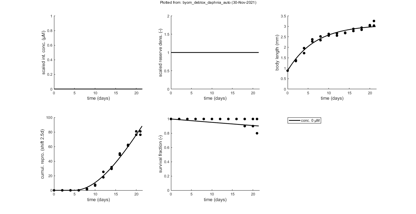
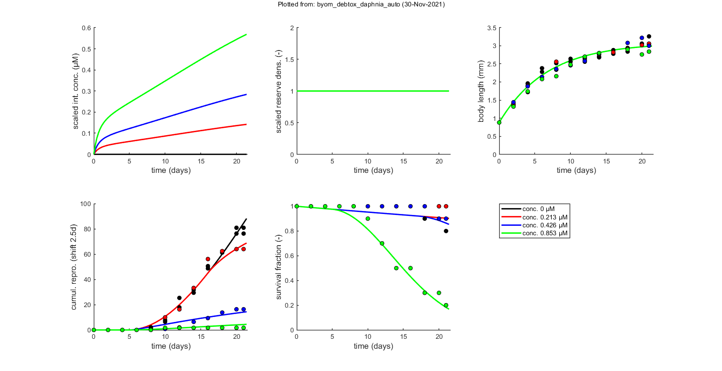
glo.stiff = [0 3]; % ODE solver 0) ode45 (standard), 1) ode113 (moderately stiff), 2) ode15s (stiff)
% Second argument is for normally tight (1), tighter (2), or very tight (3)
% tolerances. Use 1 for quick analyses, but check with 3 to see if there is
% a difference! Especially for time-varying exposure, there can be large
% differences between the settings!
glo.break_time = 0; % break time vector up for ODE solver (1) or don't (0)
% Note: breaking the time vector is a good idea when the exposure scenario
% contains discontinuities. Don't use for continuous splines (type 1) as it
% will be much slower. For FOCUS scenarios (high time resolution), breaking
% up is not efficient and does not appear to be necessary.

opt_optim.fit    = 1; % fit the parameters (1), or don't (0)
opt_optim.it     = 0; % show iterations of the optimisation (1, default) or not (0)
opt_plot.bw      = 0; % if set to 1, plots in black and white with different plot symbols
opt_plot.annot   = 2; % annotations in multiplot for fits: 1) box with parameter estimates 2) single legend
% opt_plot.statsup = [1 2]; % vector with states to suppress in plotting fits

% The switch fit_tox is used to select whether to fit the control treatment
% (0), the toxicity treatments (1; the control is shown as well), or both
% together (2). A good strategy is to fit the basic parameters to the
% control data first (fit_tox=0), copy the best values into the parameter
% matrix above, and then fit the toxicity parameter to the complete data
% set (fit_tox=1). The code below automatically does that.

skip_sg = 1; % set to 1 to skip startgrid completely (use ranges in <par> structure)
% Note: this is needed here since startgrid is currently only compatible
% with the DEBtox2019 package. You can still use the parameter-space
% explorer ...

% ===== FITTING CONTROLS ==================================================
% Simplex fitting works fine for control data. Note that hb is fitted along
% with the other parameters.
opt_optim.type = 1; % optimisation method: 1) default simplex, 4) parspace explorer
fit_tox = 0; % Fit control parameters in data set
par_out = automatic_runs_basic(fit_tox,par,ind_tox,skip_sg,opt_optim,opt_plot);
% script to run the calculations and plot, automatically
par = copy_par(par,par_out,1); % copy fitted parameters into par, and keep fit mark in par

% ===== FITTING TOX DATA ==================================================
% Here, we use the parameter-space explorer for fitting the treatments.
% Note that, with fit_tox=1, the tox parameters in par are replaced (when
% fitted) with estimates based on the data set using startgrid_debtox
% (called in automatic_runs). This is still quite experimental, so you may
% need to restart with manually-adapted ranges! Furthermore, this is really
% slow ...

opt_optim.type     = 4; % optimisation method 1) simplex, 4 parameter-space explorer
opt_optim.ps_saved = 0; % use saved set for parameter-space explorer (1) or not (0);
opt_optim.ps_plots = 0; % when set to 1, makes intermediate plots of parameter space to monitor progress
opt_optim.ps_profs = 0; % when set to 1, makes profiles and additional sampling for parameter-space explorer
opt_optim.ps_rough = 1; % set to 1 for rough settings of parameter-space explorer, 0 for settings as in openGUTS

fit_tox = 1; % Fit tox parameters in data set
par_out = automatic_runs_basic(fit_tox,par,ind_tox,skip_sg,opt_optim,opt_plot);
disp_settings_debtox2019 % display some information on the settings on screen

% dedicated TKTD plots; these plots are more readable, especially when plotting CIs
opt_tktd.repls = 0; % plot individual replicates (1) or means (0)
if opt_optim.type == 4    % when the parspace explorer was used, we can plot with CIs ...
    opt_conf.type    = 3; % make intervals from parspace explorer
    opt_conf.lim_set = 2; % use limited set of n_lim points (1) or outer hull (2) to create CIs
    plot_tktd(par_out,opt_tktd,opt_conf);
else
    plot_tktd(par_out,opt_tktd,[]); % leave the options opt_conf empty to suppress all CIs for these plots
    % Note: plotting CIs requires a sample as saved by the various
    % methods available in BYOM (see examples directory).
end
Goodness-of-fit measures for each state and each data set (R-square)
Based on the individual replicates, accounting for transformations, and including t=0
state 1.    NaN
state 2.    NaN
state 3.   0.97
state 4.   0.99
state 5.  -0.34
Warning: R-square is not appropriate for survival data so interpret
qualitatively!
Warning: (R-square not calculated when missing/removed animals; use plot_tktd)

=================================================================================
Results of the parameter estimation with BYOM (par-engine) version 6.0 BETA 7
=================================================================================
   Filename      : byom_debtox_daphnia_auto
   Analysis date : 30-Nov-2021 (12:34)
   Data entered  :
     data state 1: 0x0, no data.
     data state 2: 0x0, no data.
     data state 3: 12x5, continuous data, no transf.
     data state 4: 12x5, continuous data, no transf.
     data state 5: 12x5, survival data.
   Search method: Nelder-Mead simplex direct search, 2 rounds.
     The optimisation routine has converged to a solution
     Total 255 simplex iterations used to optimise.
     Minus log-likelihood has reached the value 178.99 (AIC=367.98).
=================================================================================
L0           0.88 (fit: 0, initial: 0.88)
Lp          1.625 (fit: 1, initial: 1.6)
Lm          3.081 (fit: 1, initial: 3.1)
rB         0.1499 (fit: 1, initial: 0.14)
Rm          9.865 (fit: 1, initial: 11)
g           0.422 (fit: 0, initial: 0.422)
f               1 (fit: 0, initial:  1)
h0       0.004813 (fit: 1, initial: 0.0024)
ke          0.039 (fit: 0, initial: 0.039)
c0          0.063 (fit: 0, initial: 0.063)
cT          0.007 (fit: 0, initial: 0.007)
c0s          0.15 (fit: 0, initial: 0.15)
b             1.1 (fit: 0, initial: 1.1)
=================================================================================
Mode of action used: 4
=================================================================================
Time required: 5.0 secs
Plots result from the optimised parameter values.
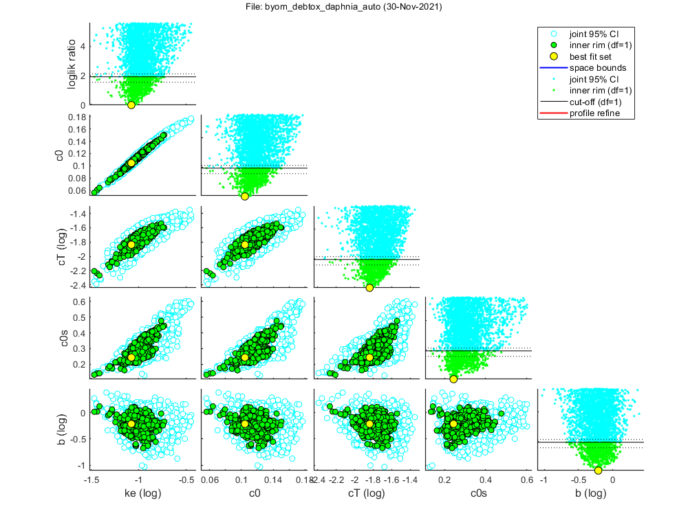
par.Lp     = [    1.6253  1      0.001        100 1];
par.Lm     = [    3.0813  1      0.001        100 1];
par.rB     = [    0.1499  1          0        100 1];
par.Rm     = [     9.865  1          0      1e+06 1];
par.h0     = [ 0.0048132  1          0      1e+06 1];
Warning: The parameter-space explorer is not thoroughly tested for more than 4
free parameters!

Settings for parameter search ranges:
=====================================================================
L0    fixed :       0.88              fit: 0
Lp    fixed :      1.625              fit: 0
Lm    fixed :      3.081              fit: 0
rB    fixed :     0.1499              fit: 0
Rm    fixed :      9.865              fit: 0
g     fixed :      0.422              fit: 0
f     fixed :          1              fit: 0
h0    fixed :   0.004813              fit: 0
ke    bounds:       0.01 -         10 fit: 1 (log)
c0    bounds:          0 -        0.8 fit: 1 (norm)
cT    bounds:     0.0001 -         10 fit: 1 (log)
c0s   bounds:          0 -        0.8 fit: 1 (norm)
b     bounds:      0.001 -         10 fit: 1 (log)
=====================================================================
Mode of action: 4
Using latin-hypercube sampling in first round, instead of regular grid.

Starting round 1 with initial grid of 10000 parameter sets
  Status: best fit so far is (minloglik) 507.6212
Starting round 2, refining a selection of 400 parameter sets, with 25 tries each
  Status: 9 sets within total CI and 8 within inner. Best fit: 502.1904
Starting round 3, refining a selection of 400 parameter sets, with 25 tries each
  Status: 17 sets within total CI and 16 within inner. Best fit: 501.9185
Starting round 4, refining a selection of 400 parameter sets, with 25 tries each
  Status: 75 sets within total CI and 30 within inner. Best fit: 501.9185
Starting round 5, refining a selection of 400 parameter sets, with 25 tries each
  Status: 540 sets within total CI and 103 within inner. Best fit: 501.9185
Starting round 6, refining a selection of 675 parameter sets, with 10 tries each
  Status: 1612 sets within total CI and 269 within inner. Best fit: 501.9185
  Next round will focus on inner rim (outer rim has enough points)
Starting round 7, refining a selection of 400 parameter sets, with 10 tries each
  Status: 3164 sets within total CI and 764 within inner. Best fit: 501.9185
  Finished sampling, running a simplex optimisation ...
  Status: 3164 sets within total CI and 764 within inner. Best fit: 501.9168
Results from the limited parspace exploration (initial sampling only).
This can be copied-pasted into your BYOM script.
Warning: for oddly-shaped parameter spaces, this may miss local minima!
(in extreme cases, even the global optimum can be missed)
Suggestions for min-max search bounds returned in par_out.
=======================================================================
par.ke     = [  0.083591  1   0.028315    0.42918 0];
par.c0     = [   0.10448  1   0.046754    0.21255 1];
par.cT     = [  0.014501  1  0.0033956   0.053515 0];
par.c0s    = [   0.24422  1    0.10811    0.72078 1];
par.b      = [   0.61285  1   0.077474     2.9066 0];
=======================================================================

=================================================================================
Results of the parameter-space exploration
=================================================================================
   Sample: 3164 sets in joint CI and 764 in inner CI.
   Propagation set: 388 sets will be used for error propagation.
Best estimates and 95% CIs on fitted parameters
Rough settings were used.
  In almost all cases, this will be sufficient for reliable results.
Profiling and additional sampling steps were skipped.
  CIs below are just the edges of the inner cloud (underestimating the true CIs).
  Advised search ranges above are derived from approx. CIs +- 20%.
==========================================================================
ke    best:    0.08359 (   0.03398  -    0.1858 ) fit: 1 (log)
c0    best:     0.1045 (   0.05620  -    0.1508 ) fit: 1 (norm)
cT    best:    0.01450 (  0.004713  -   0.03046 ) fit: 1 (log)
c0s   best:     0.2442 (    0.1342  -    0.4761 ) fit: 1 (norm)
b     best:     0.6128 (    0.2115  -     1.327 ) fit: 1 (log)
==========================================================================

Goodness-of-fit measures for each state and each data set (R-square)
Based on the individual replicates, accounting for transformations, and including t=0
state 1.    NaN
state 2.    NaN
state 3.   0.97
state 4.   0.99
state 5.   0.91
Warning: R-square is not appropriate for survival data so interpret
qualitatively!
Warning: (R-square not calculated when missing/removed animals; use plot_tktd)

=================================================================================
Results of the parameter estimation with BYOM (par-engine) version 6.0 BETA 7
=================================================================================
   Filename      : byom_debtox_daphnia_auto
   Analysis date : 30-Nov-2021 (12:44)
   Data entered  :
     data state 1: 0x0, no data.
     data state 2: 0x0, no data.
     data state 3: 12x5, continuous data, no transf.
     data state 4: 12x5, continuous data, no transf.
     data state 5: 12x5, survival data.
   Search method: Parameter-space explorer (see CIs above).
     The optimisation routine has converged to a solution
     Minus log-likelihood has reached the value 501.92 (AIC=1013.83).
=================================================================================
L0           0.88 (fit: 0, initial: NaN)
Lp          1.625 (fit: 0, initial: NaN)
Lm          3.081 (fit: 0, initial: NaN)
rB         0.1499 (fit: 0, initial: NaN)
Rm          9.865 (fit: 0, initial: NaN)
g           0.422 (fit: 0, initial: NaN)
f               1 (fit: 0, initial: NaN)
h0       0.004813 (fit: 0, initial: NaN)
ke        0.08359 (fit: 1, initial: NaN)
c0         0.1045 (fit: 1, initial: NaN)
cT        0.01450 (fit: 1, initial: NaN)
c0s        0.2442 (fit: 1, initial: NaN)
b          0.6128 (fit: 1, initial: NaN)
=================================================================================
Parameters ke, cT and b are fitted on log-scale.
=================================================================================
Mode of action used: 4
=================================================================================
Time required: 10 mins, 24.2 secs
Plots result from the optimised parameter values.
========================================================================
Extra information on the model fit (DEBtox2019, stdDEB or extended GUTS)
Mode of action        : 4

Model and ODE solver ----------------------------------------------
   Breaking time vector in call_deri: 0
   Settings for ODE solver call_deri: 0  3
   Brood-pouch delay for model (d)  : 2.5
Options for parspace explorer -------------------------------------
   Rough settings (recommended: 1)  : 1
   Make profile likelihoods         : 0
Options for startgrid ---------------------------------------------
   Skip automatic startgrid ranges  : 1
===================================================================

Plot_tktd uses uses parameter set from user input for best-fit curves.
Plot_tktd uses complete parameter set from user input for best-fit curves, but CIs use all parameters from saved set.
This may lead to strange results if the input par does not result from the same fit as the saved file
(CIs may not correspond to the best curve), so interpret with care.

Amount of 0.3764 added to the chi-square criterion for inner rim
Slightly more is taken to provide a generally conservative estimate of the CIs.
  Outer hull of 387 sets used.
Calculating CIs on model predictions, using sample from parspace explorer ... please be patient.

Warning: Boundaries of parameters in the saved set differ from that in the
workspace.
         (differences in log-settings or boundaries can be expected in various analyses)

Time required: 10 mins, 29.5 secs
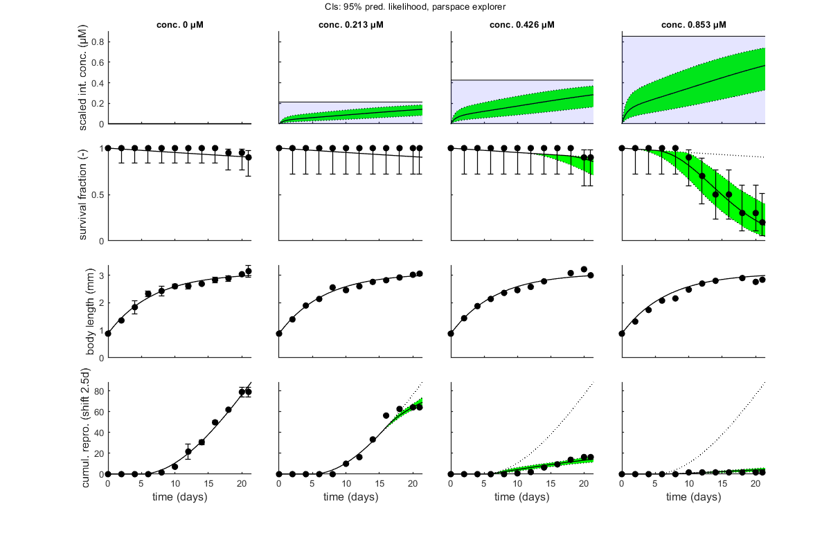
Goodness-of-fit metrics (treat with caution!)
 Values below are calculated on means, incl. t=0, from the residuals
 Residuals are used without accounting for any transformations
 However, means are calculated with transformation (if specified in DATA)

            Model efficiency (r2)   NRMSE
================================================================================
  survival    : 0.9363              0.0551
  body length : 0.9764              0.0437
  reproduction: 0.9863              0.1872
================================================================================
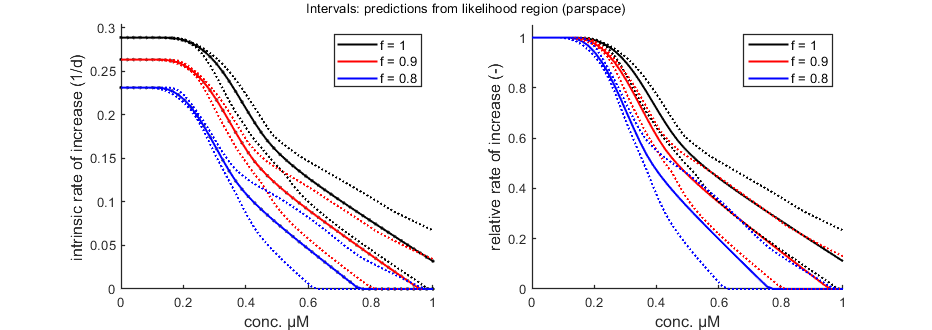
Population growth rate
The function calc_pop allows for a calculation of the intrinsic rate of population increase (Euler-Lotka equation). It calculates the growth rate at three food levels (set in the engine file calc_pop.m).
% Population calculations can be performed with CIs
opt_conf.type    = 3; % make intervals from 1) slice sampler, 2)likelihood region, 3) parspace explorer
opt_conf.lim_set = 2; % for lik-region sample: use limited set of n_lim points (1) or outer hull (2) to create CIs

Tpop = linspace(0,42,100); % time vector for the population calculations
Cpop = linspace(0,1,50);   % concentration range for population calculations
% Cpop = -1; % use only concentrations as given in X0mat
Th = glo.Tbp; % time from fresh egg to t=0 in time vector (e.g., hatching time)
% Here, use glo.Tbp days, as this value was earlier subtracted from the
% time vector in the data set. So, reproduction now represents egg
% formation, and we need to account for hatching time in the population
% calculation.

calc_pop(par_out,X0mat,Tpop,Cpop,Th,opt_conf,opt_pop)
Amount of 0.3764 added to the chi-square criterion for inner rim
Slightly more is taken to provide a generally conservative estimate of the CIs.
  Outer hull of 387 sets used.
Calculating CIs on model predictions, using sample from parspace explorer ... please be patient.

Warning: Boundaries of parameters in the saved set differ from that in the
workspace.
         (differences in log-settings or boundaries can be expected in various analyses)

Parallel toolbox is used; no progress is shown.