BYOM, byom_debkiss_no_egg.m
- Author: Tjalling Jager
- Date: November 2021
- Web support: http://www.debtox.info/byom.html
- Back to index walkthrough_debkiss.html
BYOM is a General framework for simulating model systems in terms of ordinary differential equations (ODEs). The model itself needs to be specified in derivatives.m, and call_deri.m may need to be modified to the particular problem as well. The files in the engine directory are needed for fitting and plotting. Results are shown on screen but also saved to a log file (results.out).
The model: standard DEBkiss model (see http://www.debtox.info/book_debkiss.html) following Jager et al (2013), http://dx.doi.org/10.1016/j.jtbi.2013.03.011. Parameters on length basis, and ignoring the embryonic stage.
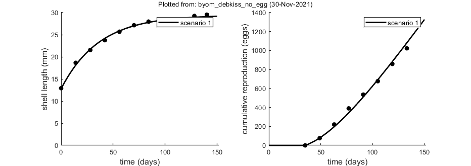
This script: Example is for the pond snail at maximum food. This is a fit to data for juvenile/adults. The data set was also used in Zimmer et al (2012), http://dx.doi.org/10.1007/s10646-012-0973-5.
Copyright (c) 2012-2021, Tjalling Jager, all rights reserved.
This source code is licensed under the MIT-style license found in the
LICENSE.txt file in the root directory of BYOM.
Contents
Initial things
Make sure that this script is in a directory somewhere below the BYOM folder.
clear, clear global % clear the workspace and globals
global DATA W X0mat % make the data set and initial states global variables
global glo          % allow for global parameters in structure glo
diary off           % turn of the diary function (if it is accidentaly on)
% set(0,'DefaultFigureWindowStyle','docked'); % collect all figure into one window with tab controls
set(0,'DefaultFigureWindowStyle','normal'); % separate figure windows

pathdefine(0) % set path to the BYOM/engine directory (option 1 uses parallel toolbox)
glo.basenm  = mfilename; % remember the filename for THIS file for the plots
glo.saveplt = 0; % save all plots as (1) Matlab figures, (2) JPEG file or (3) PDF (see all_options.txt)
The data set
Data are entered in matrix form, time in rows, scenarios (exposure concentrations) in columns. First column are the exposure times, first row are the concentrations or scenario numbers. The number in the top left of the matrix indicates how to calculate the likelihood:
- -1 for multinomial likelihood (for survival data)
- 0 for log-transform the data, then normal likelihood
- 0.5 for square-root transform the data, then normal likelihood
- 1 for no transformation of the data, then normal likelihood
% Shell length in mm over time in ad libitum feeding regime
DATA{1} = [0.5        1
            0       12.918
           14        18.65
           28       21.549
           42       23.759
           56       25.669
           70       27.146
           84       27.953
           98       28.189
          112        28.27
          128       29.242
          140        29.53];

% weight factors (number of replicates per observation)
W{1} = [30
    30
    29
    28
    28
    26
    26
    26
    25
    23
    21  ];

% Cumulative reproduction over time in ad libitum feeding regime; reduced data
DATA{2}= [0.5            1
           35            0
           49           76
           63        219.8
           77        389.7
           91        534.6
          105        676.8
          119        858.9
          133       1023.1    ];

W{2} = [28
    28
    28
    26
    26
    26
    24
    23   ];

% if weight factors are not specified, ones are assumed in start_calc.m
Initial values for the state variables
Initial states, scenarios in columns, states in rows. First row are the 'names' of all scenarios.
X0mat = [1       % the scenarios
         12.8    % initial shell length in mm
         0];     % initial cumul. repro

% Put the position of the various states in globals, to make sure correct
% one is selected for extra things (e.g., to prevent shrinking in
% call_deri, and for using plot_tktd).
glo.locL = 1; % location of body size in the state variable list
glo.locR = 2; % location of cumulative reproduction in the state variable list
Initial values for the model parameters
Model parameters are part of a 'structure' for easy reference. Global parameters as part of the structure glo
glo.delM  = 0.401; % shape corrector (used in call_deri.m)
glo.dV    = 0.1;   % dry weight density (used in call_deri.m)
glo.len   = 2;     % switch to fit physical length (0=off, 1=on, 2=on and no shrinking) (used in call_deri.m)
glo.mat   = 1;     % include maturity maint. (0=off, 1=include)
% Note: if glo.len > 0 than the initial state for size in X0mat is length too!

% syntax: par.name = [startvalue fit(0/1) minval maxval optional:log/normal scale (0/1)];
par.sJAm = [0.15    1 0 1e6]; % specific assimilation rate
par.sJM  = [0.010   1 0 1e6]; % specific maintenance costs
par.WB0  = [0.15    0 0 1e6]; % initial weight of egg
par.Lwp  = [22      1 0 1e6]; % shell length at puberty
par.yAV  = [0.8     0 0 1];   % yield of assimilates on volume (starvation)
par.yBA  = [0.95    0 0 1];   % yield of egg buffer on assimilates
par.yVA  = [0.8     0 0 1];   % yield of structure on assimilates (growth)
par.kap  = [0.79    1 0 1];   % allocation fraction to soma
par.f    = [1       0 0 2];   % scaled food leve
par.fB   = [0.5     0 0 2];   % scaled food level, embryo
par.Lwf  = [0       0 0 500]; % half-saturation shell length
Time vector and labels for plots
Specify what to plot. If time vector glo.t is not specified, a default is constructed, based on the data set.
glo.t   = linspace(0,150,100); % time vector for the model curves in days

% specify the y-axis labels for each state variable
glo.ylab{1} = 'shell length (mm)';
glo.ylab{2} = 'cumulative reproduction (eggs)';
% specify the x-axis label (same for all states)
glo.xlab    = 'time (days)';
glo.leglab1 = 'scenario '; % legend label before the 'scenario' number
glo.leglab2 = ''; % legend label after the 'scenario' number

prelim_checks % script to perform some preliminary checks and set things up
% Note: prelim_checks also fills all the options (opt_...) with defauls, so
% modify options after this call, if needed.
Calculations and plotting
Here, the function is called that will do the calculation and the plotting. Options for the plotting can be set using opt_plot (see prelim_checks.m). Options for the optimsation routine can be set using opt_optim. Options for the ODE solver are part of the global glo.
NOTE: for this package, the options useode and eventson in glo will not be functional: the ODE solver is always used, and the events function as well.
For the demo, the iterations are turned off (opt_optim.it = 0).
glo.stiff = [0 3]; % ODE solver 0) ode45 (standard), 1) ode113 (moderately stiff), 2) ode15s (stiff)
% Second argument is for normally tight (1), tighter (2), or very tight (3)
% tolerances. Use 1 for quick analyses, but check with 3 to see if there is
% a difference!

opt_optim.fit    = 1; % fit the parameters (1), or don't (0)
opt_optim.it     = 0; % show iterations of the optimisation (1, default) or not (0)
opt_plot.bw      = 0; % if set to 1, plots in black and white with different plot symbols
opt_plot.annot   = 0; % annotations in multiplot for fits: 1) box with parameter estimates 2) single legend

% optimise and plot (fitted parameters in par_out)
par_out = calc_optim(par,opt_optim); % start the optimisation
calc_and_plot(par_out,opt_plot); % calculate model lines and plot them

% % Code below demonstrates the use of the new plotting routine. However,
% % since we have only a single treatment here, the added benefit is not so
% % great.
% opt_tktd.repls = 0; % plot individual replicates (1) or means (0)
% opt_tktd.obspred = 0; % plot predicted-observed plots (1) or not (0), (2) makes 1 plot for multiple data sets
% plot_tktd(par_out,opt_tktd,[]);
% % Leave the options opt_conf empty to suppress all CIs for these plots.
% % Plotting CIs requires a sample as saved by the various methods available
% % in BYOM (see examples directory).
Goodness-of-fit measures for each state and each data set (R-square)
Based on the individual replicates, accounting for transformations, and including t=0
state 1.   1.00
state 2.   1.00
=================================================================================
Results of the parameter estimation with BYOM version 6.0 BETA 7
=================================================================================
   Filename      : byom_debkiss_no_egg
   Analysis date : 30-Nov-2021 (10:51)
   Data entered  :
     data state 1: 11x1, continuous data, power 0.50 transf.
     data state 2: 8x1, continuous data, power 0.50 transf.
   Search method: Nelder-Mead simplex direct search, 2 rounds.
     The optimisation routine has converged to a solution
     Total 295 simplex iterations used to optimise.
     Minus log-likelihood has reached the value 51.92 (AIC=111.83).
=================================================================================
sJAm       0.1545 (fit: 1, initial: 0.15)
sJM       0.01028 (fit: 1, initial: 0.01)
WB0          0.15 (fit: 0, initial: 0.15)
Lwp         23.07 (fit: 1, initial: 22)
yAV           0.8 (fit: 0, initial: 0.8)
yBA          0.95 (fit: 0, initial: 0.95)
yVA           0.8 (fit: 0, initial: 0.8)
kap        0.7859 (fit: 1, initial: 0.79)
f               1 (fit: 0, initial:  1)
fB            0.5 (fit: 0, initial: 0.5)
Lwf             0 (fit: 0, initial:  0)
=================================================================================
Time required: 4.4 secs
Plots result from the optimised parameter values.
Profiling the likelihood
By profiling you make robust confidence intervals for one or more of your parameters. Use the names of the parameters as they occurs in your parameter structure par above. This can be a single string (e.g., 'kd'), a cell array of strings (e.g., {'rB','Lm'}), or 'all' to profile all fitted parameters. If you have used the parameter-space explorer for fitting, you already have (even more robust) profiles!
Options for the profiling can be set using opt_prof (see prelim_checks). For this demo, the level of detail of the profiling is set to 'coarse' and no sub-optimisations are used. However, consider these options when working on your own data (e.g., set opt_prof.subopt=10).
opt_prof.detail   = 2; % detailed (1) or a coarse (2) calculation
opt_prof.subopt   = 0; % number of sub-optimisations to perform to increase robustness
opt_prof.brkprof  = 2; % when a better optimum is located, stop (1) or automatically refit (2)

calc_proflik(par_out,{'sJAm','sJM'},opt_prof,opt_optim);  % calculate a profile
% Enter single parameter names, a cell array of names, or 'all' to profile
% all fitted parameters.
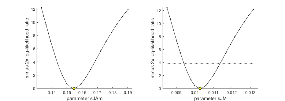
95% confidence interval(s) from the profile(s)
=================================================================================
sJAm       interval:     0.1438 -  0.1679
sJM        interval:   0.009407 -  0.01136
=================================================================================

Time required: 1 min, 24.3 secs
Other files: derivatives
To archive analyses, publishing them with Matlab is convenient. To keep track of what was done, the file derivatives.m can be included in the published result.
%% BYOM function derivatives.m (the model in ODEs)
%
%  Syntax: dX = derivatives(t,X,par,c,glo)
%
% This function calculates the derivatives for the model system. It is
% linked to the script files <byom_debkiss_no_egg.html
% byom_debkiss_no_egg.m>. As input, it gets:
%
% * _t_   is the time point, provided by the ODE solver
% * _X_   is a vector with the previous value of the states
% * _par_ is the parameter structure
% * _c_   is the external concentration (or scenario number)
% * _glo_ is the structure with information (normally global)
%
% Time _t_ and scenario name _c_ are handed over as single numbers by
% <call_deri.html call_deri.m> (you do not have to use them in this
% function). Output _dX_ (as vector) provides the differentials for each
% state at _t_.
%
% * Author: Tjalling Jager
% * Date: November 2020
% * Web support: <http://www.debtox.info/byom.html>
% * Back to index <walkthrough_debkiss.html>

%  Copyright (c) 2012-2021, Tjalling Jager, all rights reserved.
%  This source code is licensed under the MIT-style license found in the
%  LICENSE.txt file in the root directory of BYOM.

%% Start

function dX = derivatives(t,X,par,c,glo)

% NOTE: glo is now no longer a global here, but passed on in the function
% call from call_deri. That saves 20% calculation time!

%% Unpack states
% The state variables enter this function in the vector _X_. Here, we give
% them a more handy name.

WV = X(1); % state 1 is the structural body mass
% cR = X(2); % state 2 is the cumulative reproduction (not used in this function)
WB = 0; % no egg phase, so egg buffer is empty

%% Unpack parameters
% The parameters enter this function in the structure _par_. The names in
% the structure are the same as those defined in the byom script file.
% The 1 between parentheses is needed as each parameter has 5 associated
% values.

dV    = glo.dV;       % dry weight density of structure
delM  = glo.delM;     % shape correction coefficient (if needed)
% delM is used to allow Lwp as a parameter instead of WVp

sJAm  = par.sJAm(1);  % specific assimilation rate
sJM   = par.sJM(1);   % specific maintenance costs
WB0   = par.WB0(1);   % initial weight of egg
Lwp   = par.Lwp(1);   % shell length at puberty
yAV   = par.yAV(1);   % yield of assimilates on volume (starvation)
yBA   = par.yBA(1);   % yield of egg buffer on assimilates
yVA   = par.yVA(1);   % yield of structure on assimilates (growth)
kap   = par.kap(1);   % allocation fraction to soma
f     = par.f(1);     % scaled food level
fB    = par.fB(1);    % scaled food level for the embryo
Lwf   = par.Lwf(1);   % half-saturation length for initial food limitation

if glo.len ~= 0 % only if the switch is set to 1 or 2!
    % Translate shell length at puberty to body weight
    WVp = dV*(Lwp * delM).^3; % initial length to initial dwt
    WVf = dV*(Lwf * delM).^3; % initial length to initial dwt
end

%% Calculate the derivatives
% This is the actual model, specified as a system of ODEs.
% Note: some unused fluxes are calculated because they may be needed for
% future modules (e.g., respiration and ageing).

L = (WV/dV)^(1/3); % volumetric length

% Select what to do with maturity maintenance
if glo.mat == 1
    sJJ = sJM * (1-kap)/kap; % add specific maturity maintenance with the suggested value
else
    sJJ = 0; % or ignore it
end

WVb = WB0 *yVA * kap; % body mass at birth

if WB > 0 % if we have an embryo
    f = fB; % assimilation at different rate
else
    if WVf > 0
        f = f / (1+WVf/WV); % hyperbolic relationship for f with body weight
    end
end

JA = f * sJAm * L^2;          % assimilation
JM = sJM * L^3;               % somatic maintenance
JV = yVA * (kap*JA-JM);       % growth

if WV < WVp                   % below size at puberty
    JR = 0;                   % no reproduction
    JJ = sJJ * L^3;           % maturity maintenance flux
    % JH = (1-kap) * JA - JJ; % maturation flux (not used!)
else
    JJ = sJJ * (WVp/dV);      % maturity maintenance
    JR = (1-kap) * JA - JJ;   % reproduction flux
end

% Starvation rules may override these fluxes
if kap * JA < JM      % allocated flux to soma cannot pay maintenance
    if JA >= JM + JJ  % but still enough total assimilates to pay both maintenances
        JV = 0;       % stop growth
        if WV >= WVp  % for adults ...
            JR = JA - JM - JJ; % repro buffer gets what's left
        else
            % JH = JA - JM - JJ; % maturation gets what's left (not used!)
        end
    elseif JA >= JM   % only enough to pay somatic maintenance
        JV = 0;       % stop growth
        JR = 0;       % stop reproduction
        % JH = 0;     % stop maturation for juveniles (not used)
        JJ = JA - JM; % maturity maintenance flux gets what's left
    else              % we need to shrink
        JR = 0;       % stop reproduction
        JJ = 0;       % stop paying maturity maintenance
        % JH = 0;     % stop maturation for juveniles (not used)
        JV = (JA - JM) / yAV; % shrink; pay somatic maintenance from structure
    end
end

% We do not work with a repro buffer here, so a negative JR does not make
% sense; therefore, minimise to zero
JR = max(0,JR);

% Calcululate the derivatives
dWV = JV;             % change in body mass
dcR = yBA * JR / WB0; % continuous reproduction flux
if WB > 0             % for embryos ...
    dWB = -JA;        % decrease in egg buffer
else
    dWB = 0;          % for juveniles/adults, no change
end
if WV < WVb/4 && dWB == 0 % dont shrink below quarter size at birth
    dWV = 0; % simply stop shrinking ...
end

dX = [dWV;dcR];       % collect both derivatives in one vector
Other files: call_deri
To archive analyses, publishing them with Matlab is convenient. To keep track of what was done, the file call_deri.m can be included in the published result.
%% BYOM function call_deri.m (calculates the model output)
%
%  Syntax: [Xout,TE,Xout2,zvd] = call_deri(t,par,X0v,glo)
%
% This function calls the ODE solver to solve the system of differential
% equations specified in <derivatives.html derivatives.m>. As input, it
% gets:
%
% * _t_   the time vector
% * _par_ the parameter structure
% * _X0v_   a vector with initial states and one concentration (scenario number)
% * _glo_ is the structure with information (normally global)
%
% The output _Xout_ provides a matrix with time in rows, and states in
% columns. This function calls <derivatives.html derivatives.m>. The
% optional output _TE_ is the time at which an event takes place (specified
% using the events function). The events function is set up to catch
% discontinuities. It should be specified according to the problem you are
% simulating. If you want to use parameters that are (or influence) initial
% states, they have to be included in this function.
%
% * Author: Tjalling Jager
% * Date: November 2021
% * Web support: <http://www.debtox.info/byom.html>
% * Back to index <walkthrough_debkiss.html>

%  Copyright (c) 2012-2021, Tjalling Jager, all rights reserved.
%  This source code is licensed under the MIT-style license found in the
%  LICENSE.txt file in the root directory of BYOM.

%% Start

function [Xout,TE,Xout2,zvd] = call_deri(t,par,X0v,glo)

% These outputs need to be defined, even if they are not used
Xout2    = []; % additional uni-variate output, not used in this example
zvd      = []; % additional zero-variate output, not used in this example

% NOTE: this file is modified so that data and output can be as body length
% whereas the state variable remains body weight. Also, there is a
% calculation to prevent shrinking in physical length (as shells, for
% example, do not shrink).

%% Initial settings
% This part extracts optional settings for the ODE solver that can be set
% in the main script (defaults are set in prelim_checks). Further in this
% section, initial values can be determined by a parameter (overwrite parts
% of X0), and zero-variate data can be calculated. See the example BYOM
% files for more information.
%
% This package will always use the ODE solver; therefore the general
% settings in the global glo for the calculation (useode and eventson) are
% removed here. This packacge also always uses the events function, so the
% option eventson is not used. Furthermore, simplefun.m is removed.

stiff = glo.stiff; % ODE solver 0) ode45 (standard), 1) ode113 (moderately stiff), 2) ode15s (stiff)
min_t = 500; % minimum length of time vector (affects ODE stepsize only, when needed)

if length(stiff) == 1
    stiff(2) = 1; % by default: normally tightened tolerances
end

% Unpack the vector X0v, which is X0mat for one scenario
X0 = X0v(2:end); % these are the intitial states for a scenario

% % if needed, extract parameters from par that influence initial states in X0
% % start from specified initial size
% Lw0 = par.Lw0(1);  % initial body length (mm)
% X0(glo.locL) = glo.dV*((Lw0*glo.delM)^3); % recalculate to dwt, and put this parameter in the correct location of the initial vector

% start from the value provided in X0mat
if glo.len ~= 0 % only if the switch is set to 1 or 2!
    % Assume that X0mat includes initial length; if it includes mass, no correction is needed here
    % The model is set up in masses, so we need to translate the initial length
    % (in mm body length) to body mass using delM.
    X0(glo.locL) = glo.dV*((X0(glo.locL) * glo.delM)^3); % initial length to initial dwt
end

% % start at hatching, so calculate initial length from egg weight
% WB0   = par.WB0(1);     % initial dry weight of egg
% yVA   = par.yVA(1);     % yield of structure on assimilates (growth)
% kap   = par.kap(1);     % allocation fraction to soma
% WVb   = WB0 *yVA * kap; % dry body mass at birth
% X0(glo.locL) = WVb;     % put this estimate in the correct location of the initial vector

% % if needed, calculate model values for zero-variate data from parameter set
% if ~isempty(zvd)
%     zvd.ku(3) = par.Piw(1) * par.ke(1); % add model prediction as third value
% end

%% Calculations
% This part calls the ODE solver to calculate the output (the value of the
% state variables over time). There is generally no need to modify this
% part. The solver ode45 generally works well. For stiff problems, the
% solver might become very slow; you can try ode15s instead.

c     = X0v(1); % the concentration (or scenario number)
t     = t(:);   % force t to be a row vector (needed when useode=0)
t_rem = t;      % remember the original time vector (as we might add to it)

% This is a means to include a delay caused by the brood pounch in species
% like Daphnia. The repro data are for the appearance of neonates, but egg
% production occurs earlier. This global shifts the model output in this
% function below. This way, the time vector in the data does not need to be
% manipulated, and the model plots show the neonate production as expected.
% (NEW)
bp = 0; % by default, no brood-pouch delay
if isfield(glo,'Tbp') && glo.Tbp > 0 % if there is a global specifying a brood-pouch delay ...
    tbp = t(t>glo.Tbp)-glo.Tbp; % extra times needed to calculate brood-pounch delay
    t   = unique([t;tbp]);      % add the shifted time points to account for brood-pouch delay
    bp  = 1;                    % signal rest of code that we need brood-pouch delay
end

% When an animal cannot shrink in length, we need a long time vector as we
% need to catch the maximum length over time.
if glo.len == 2 && length(t) < min_t % make sure there are at least min_t points
    t = unique([t;(linspace(t(1),t(end),min_t))']);
end

% specify options for the ODE solver
options = odeset; % start with default options
% Note: since odeset takes considerable time, it is smart to set all
% options in ONE call below.

% This needs further study ...
switch stiff(2)
    case 1 % for ODE15s, slightly tighter tolerances seem to suffice (for ODE113: not tested yet!)
        options = odeset(options,'Events',@eventsfun,'RelTol',1e-4,'AbsTol',1e-7); % specify tightened tolerances
    case 2 % somewhat tighter tolerances ...
        options = odeset(options,'Events',@eventsfun,'RelTol',1e-5,'AbsTol',1e-8); % specify tightened tolerances
    case 3 % for ODE45, very tight tolerances seem to be necessary
        options = odeset(options,'Events',@eventsfun,'RelTol',1e-9,'AbsTol',1e-9); % specify MORE tightened tolerances
end
% Note: setting tolerances is pretty tricky. For some cases, tighter
% tolerances are needed but not for others. For ODE45, tighter tolerances
% seem to work well, but not for ODE15s.

% The code below uses an ODE solver to go through the time vector in one
% run. The DEBtox packages use code that can break up the time vector in
% sections. That would be especially useful if conditions change
% (non-smoothly) over time. But here, we keep things simple.

TE = 0; % dummy for time of events
% call the ODE solver with an events functions ... additional output arguments for events:
% TE catches the time of an event
switch stiff(1)
    case 0
        [tout,Xout,TE,~,~] = ode45(@derivatives,t,X0,options,par,c,glo);
    case 1
        [tout,Xout,TE,~,~] = ode113(@derivatives,t,X0,options,par,c,glo);
    case 2
        [tout,Xout,TE,~,~] = ode15s(@derivatives,t,X0,options,par,c,glo);
end

if isempty(TE) || all(TE == 0) % if there is no event caught
    TE = +inf; % return infinity
end

%% Output mapping
% _Xout_ contains a row for each state variable. It can be mapped to the
% data. If you need to transform the model values to match the data, do it
% here.

% here, translate from the state body weight to output in length, if needed
if glo.len ~= 0 % only if the switch is set to 1 or 2!
    % Here, I translate the model output in body mass to estimated physical body length
    W = Xout(:,glo.locL); % take dry body weight from the correct location in Xout
    L = (W/glo.dV).^(1/3)/glo.delM; % estimated physical body length

    if glo.len == 2 % when animal cannot shrink in length (but does on volume!)
        L = cummax(L); % replace L by the maximum achieved over time
    end
    Xout(:,glo.locL) = L; % replace body weight by physical body length
end

if bp == 1 % if we need a brood-pouch delay ... (NEW)
    [~,loct] = ismember(tbp,tout); % find where the extra brood-pouch time points are in the long Xout
    Xbp      = Xout(loct,glo.locR); % only keep the brood-pouch ones we asked for
end
t = t_rem; % return t to the original input vector

% Select the correct time points to return to the calling function
[~,loct] = ismember(t,tout); % find where the requested time points are in the long Xout
Xout     = Xout(loct,:);     % only keep the ones we asked for

if bp == 1 % if we need a brood-pouch delay ... (NEW)
    [~,loct] = ismember(tbp+glo.Tbp,t); % find where the extra brood-pouch time points SHOULD BE in the long Xout
    Xout(:,glo.locR)    = 0;   % clear the reproduction state variable
    Xout(loct,glo.locR) = Xbp; % put in the brood-pouch ones we asked for
end

% % To obtain the output of the derivatives at each time point. The values in
% % dXout might be used to replace values in Xout, if the data to be fitted
% % are the changes (rates) instead of the state variable itself.
% % dXout = zeros(size(Xout)); % initialise with zeros
% for i = 1:length(t) % run through all time points
%     dXout(i,:) = derivatives(t(i),Xout(i,:),par,c,glo);
%     % derivatives for each stage at each time
% end

%% Events function
% This subfunction catches the 'events': in this case, it looks for birth
% and the point where size exceeds the threshold for puberty. This function
% should be adapted to the problem you are modelling.
%
% Note that the eventsfun has the same inputs, in the same sequence, as
% <derivatives.html derivatives.m>.

function [value,isterminal,direction] = eventsfun(t,X,par,c,glo)

% Note: glo needs to be an input to the events function as well, rather
% than a global since the inputs for the events function must match those
% for derivatives.

Lwp      = par.Lwp(1); % shell length at puberty
if glo.len ~= 0 % only if the switch is set to 1 or 2!
    % Translate shell length at puberty to body weight
    WVp = glo.dV*(Lwp * glo.delM).^3; % initial length to initial dwt
end

nevents  = 1;          % number of events that we try to catch

value       = zeros(nevents,1);  % initialise with zeros
value(1)    = X(glo.locL) - WVp; % thing to follow is body mass (state 1) minus threshold

isterminal  = zeros(nevents,1); % do NOT stop the solver at an event
direction   = zeros(nevents,1); % catch ALL zero crossing when function is increasing or decreasing