BYOM, byom_bioconc_sim.m, simulator example

BYOM is a General framework for simulating model systems in terms of ordinary differential equations (ODEs). The model itself needs to be specified in derivatives.m, and call_deri.m may need to be modified to the particular problem as well. The files in the engine directory are needed for fitting and plotting. Results are shown on screen but also saved to a log file (results.out).

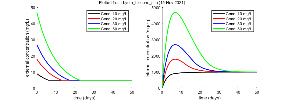
The model: An organism is exposed to a chemical in its surrounding medium. The animal accumulates the chemical according to standard one-compartment first-order kinetics, specified by a bioconcentration factor (Piw) and an elimination rate (ke). The chemical degrades at a certain rate (kd). When the external concentration reaches a certain concentration (Ct), degradation stops.

This script: byom_bioconc_sim is an example of how to use the simulator. If you start building a model, simulations are useful to get a better idea of what the model can do. By all means also try plot_option = 5 (plots the derivative versus the state variable). Make sure that the ODE version of the model is used (set useode=1 in call_deri.m).

Copyright (c) 2012-2021, Tjalling Jager, all rights reserved.
This source code is licensed under the MIT-style license found in the
LICENSE.txt file in the root directory of BYOM.

Contents

Initial things

Make sure that this script is in a directory somewhere below the BYOM folder.

clear, clear global % clear the workspace and globals
global X0mat        % make scenarios global
global glo          % allow for global parameters in structure glo
diary off           % turn off the diary function (if it is accidentaly on)
% set(0,'DefaultFigureWindowStyle','docked'); % collect all figure into one window with tab controls
set(0,'DefaultFigureWindowStyle','normal'); % separate figure windows

pathdefine % set path to the BYOM/engine directory
glo.basenm = mfilename; % remember the filename for THIS file for the plots

Initial values for the state variables

Initial states, scenarios in columns, states in rows. First row are the 'names' of all scenarios.

X0mat = [10 20 30 50    % the scenarios (here nominal concentrations)
          9 18 27 47    % initial values state 1 (actual external concentrations)
          0  0  0  0];  % initial values state 2 (internal concentrations)

Initial values for the model parameters

Model parameters are part of a 'structure' for easy reference.

% syntax: par.name = [startvalue];
par.kd    = 0.1;  % degradation rate constant, d-1
par.ke    = 0.2;  % elimination rate constant, d-1
par.Piw   = 200;  % bioconcentration factor, L/kg
par.Ct    = 5;    % threshold external concentration where degradation stops, mg/L

What to calculate and what to plot

Specify what to calculate and what to plot.

glo.t = linspace(0,50,100); % time vector for the model curves in days

% specify the y-axis labels for each state variable
glo.ylab{1} = 'external concentration (mg/L)';
glo.ylab{2} = 'internal concentration (mg/kg)';
% specify the x-axis label (same for all states)
glo.xlab    = 'time (days)';
glo.leglab1 = 'Conc. '; % legend label before the 'scenario' number
glo.leglab2 = ' mg/L'; % legend label after the 'scenario' number

% set options for call_deri here (we don't do prelim_checks for simulations)
glo.useode   = 1; % calculate model using ODE solver (1)
glo.eventson = 1; % events function on (1) or off (0)
glo.stiff    = 0; % set to 1 to use a stiff solver instead of the standard one
glo.zvd      = []; % this is normally done in prelim_checks, but we skip that here

Optional settings

Also try plottype 5 for this example! See the SIMbyom package for more detailed information on the simulator options.

opt_sim.plottype = 3; % default: 4
% 1) 3d plot,
% 2) 2d plot,
% 3) states in subplots,
% 4) scenarios in subplots,
% 5) dx/dt versus x
% 6) 2d plot for each scenario separate

Calculations and plotting

Here, the script is called that will do the calculation and the plotting.

sim_and_plot(par,opt_sim); % call the script which calculates and plots

Local sensitivity analysis

Local sensitivity analysis of the model. All model parameters are increased one-by-one by a small percentage. The sensitivity score is by default scaled (dX/X p/dp) or alternatively absolute (dX p/dp).

Options for the sensitivity can be set using opt_sens (see prelim_checks.m).

prelim_checks % call prelim_checks to create some settings needed for the sensitivity analysis

% % UNCOMMENT LINE(S) TO CALCULATE
% opt_sens.type  = 1; % type of analysis 1) relative sensitivity 2) absolute sensitivity
% opt_sens.state = 0; % vector with state variables for the sensitivity analysis (0 does all, if sens>0)
% calc_localsens(par,opt_sens)

Published with MATLAB® R2021b