BYOM, byom_bioconc_parspace.m, a quick example
- Author: Tjalling Jager
- Date: November 2021
- Web support: http://www.debtox.info/byom.html
- Back to index walkthrough_byom.html
BYOM is a General framework for simulating model systems in terms of ordinary differential equations (ODEs). The model itself needs to be specified in derivatives.m, and call_deri.m may need to be modified to the particular problem as well. The files in the engine directory are needed for fitting and plotting. Results are shown on screen but also saved to a log file (results.out).
The model: An organism is exposed to a chemical in its surrounding medium. The animal accumulates the chemical according to standard one-compartment first-order kinetics, specified by a bioconcentration factor (Piw) and an elimination rate (ke). The chemical degrades at a certain rate (kd). When the external concentration reaches a certain concentration (Ct), degradation stops. This is useful to demonstrate the events function in call_deri.m, which catches this discontuity graciously.
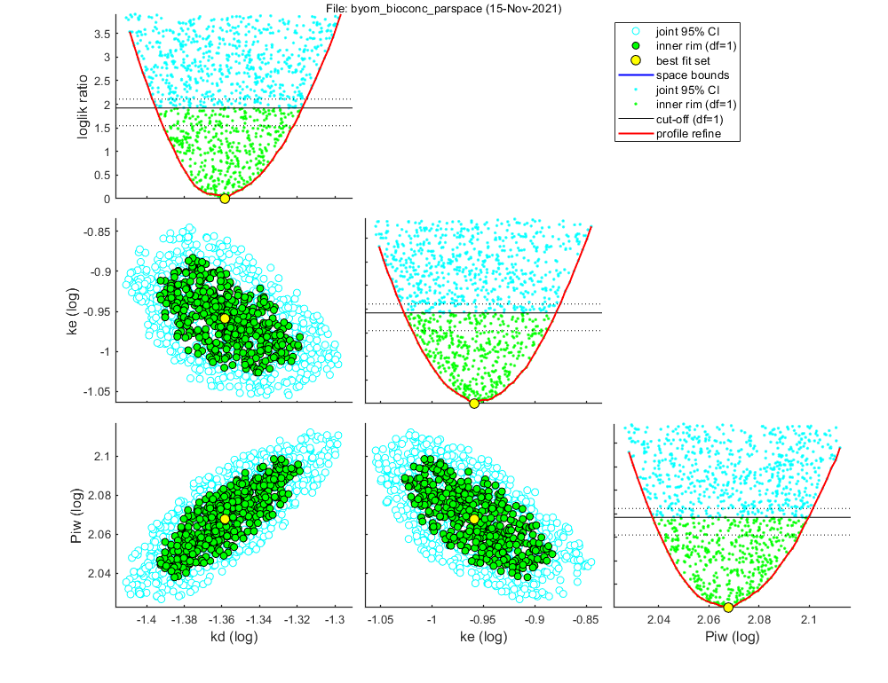
This script: byom_bioconc_parspace demonstrates the use of the openGUTS parameter-space explorer algorithm. The user needs to set search ranges, but after that, the algorithm will find the optimum, CIs on model parameters, and a sample to be used for CIs on model curves. Note that this analysis takes a bit of time to finish (some 5-8 min.). However, with the parallel toolbox it will be considerably faster (depending on how many physical cores your machine has).
Copyright (c) 2012-2021, Tjalling Jager, all rights reserved.
This source code is licensed under the MIT-style license found in the
LICENSE.txt file in the root directory of BYOM.
Contents
Initial things
Make sure that this script is in a directory somewhere below the BYOM folder.
clear, clear global % clear the workspace and globals
global DATA W X0mat % make the data set and initial states global variables
global glo          % allow for global parameters in structure glo
diary off           % turn off the diary function (if it is accidentaly on)
% set(0,'DefaultFigureWindowStyle','docked'); % collect all figure into one window with tab controls
set(0,'DefaultFigureWindowStyle','normal'); % separate figure windows

pathdefine(0) % set path to the BYOM/engine directory (option 1 to use parallel toolbox, if available)
glo.basenm  = mfilename; % remember the filename for THIS file for the plots
glo.saveplt = 0; % save all plots as (1) Matlab figures, (2) JPEG file or (3) PDF (see all_options.txt)
The data set
Data are entered in matrix form, time in rows, scenarios (exposure concentrations) in columns. First column are the exposure times, first row are the concentrations or scenario numbers. The number in the top left of the matrix indicates how to calculate the likelihood:
- -1 for multinomial likelihood (for survival data)
- 0 for log-transform the data, then normal likelihood
- 0.5 for square-root transform the data, then normal likelihood
- 1 for no transformation of the data, then normal likelihood
% observed external concentrations (two series per concentration)
DATA{1} = [ 1  10 10 20 20 30 30
            0  11 12 20 19 28 29
            10  6  8 13 12 20 18
            20  4  5  9  7 10 12
            30  5  7  6  4  6  7
            40  4  5  6  5  4  3];

% weight factors (number of replicates per observation in DATA{1})
W{1} = [10 10 10 10 10 10
        10 10 10 10 10 10
         8  8  8  8  8  9
         8  7  7  8  8  9
         6  6  6  6  6  7];

% observed internal concentrations (two series per concentration)
DATA{2} = [0.5   10  10   20   20   50   50
           0    0   0    0    0    0    0
           10 570 600 1150 1100 2500 3000
           20 610 650 1300 1210 2700 2800
           25 590 620  960  900 2300 2200
           40 580 560  920  650 1200 1700];

% if weight factors are not specified, ones are assumed in start_calc.m
Initial values for the state variables
Initial states, scenarios in columns, states in rows. First row are the 'names' of all scenarios.
X0mat = [10 20 30 50    % the scenarios (here nominal concentrations)
          9 18 27 47    % initial values state 1 (actual external concentrations)
          0  0  0  0];  % initial values state 2 (internal concentrations)
Initial values for the model parameters
Model parameters are part of a 'structure' for easy reference.
% syntax: par.name = [startvalue fit(0/1) minval maxval optional:log/normal
% scale (0/1)]; Note: when using parspace, the search ranges and the
% log/normal scale flags are very important, and need to be set with care.
% The starting-value in the first column is irrelevant, but needs to be
% within the search range.
par.kd    = [0.1  1 0.01 10   0];  % degradation rate constant, d-1
par.ke    = [0.2  1 0.01 10   0];  % elimination rate constant, d-1
par.Piw   = [200  1 10   1000 0];  % bioconcentration factor, L/kg
par.Ct    = [5    0 0    1e6  1];  % threshold external concentration where degradation stops, mg/L
Time vector and labels for plots
Specify what to plot. If time vector glo.t is not specified, a default is constructed, based on the data set.
% specify the y-axis labels for each state variable
glo.ylab{1} = 'external concentration (mg/L)';
glo.ylab{2} = 'internal concentration (mg/kg)';
% specify the x-axis label (same for all states)
glo.xlab    = 'time (days)';
glo.leglab1 = 'conc. '; % legend label before the 'scenario' number
glo.leglab2 = 'mg/L';   % legend label after the 'scenario' number

prelim_checks % script to perform some preliminary checks and set things up
% Note: prelim_checks also fills all the options (opt_...) with defauls, so
% modify options after this call, if needed.
Calculations and plotting
Here, the functions are called that will do the calculation and the plotting.
Options for the plotting can be set using opt_plot (see prelim_checks.m). Options for the optimsation routine can be set using opt_optim. Options for the ODE solver are part of the global glo. For the demo, the iterations were turned off (opt_optim.it = 0).
opt_optim.type   = 4; % optimisation method 1) simplex, 4) parameter-space explorer
opt_optim.fit    = 1; % fit the parameters (1), or don't (0)
opt_optim.it     = 1; % show iterations of the optimisation (1, default) or not (0)
opt_plot.bw      = 1; % if set to 1, plots in black and white with different plot symbols
opt_plot.annot   = 2; % annotations in multiplot for fits: 1) box with parameter estimates 2) single legend
% opt_plot.statsup = [2]; % vector with states to suppress in plotting fits

opt_optim.ps_plots = 1; % when set to 1, makes intermediate plots to monitor progress of parameter-space explorer
opt_optim.ps_profs = 1; % when set to 1, makes profiles and additional sampling for parameter-space explorer
opt_optim.ps_rough = 1; % set to 1 for rough settings of parameter-space explorer, 0 for settings as in openGUTS
opt_optim.ps_saved = 0; % use saved set for parameter-space explorer (1) or not (0);

% optimise and plot (fitted parameters in par_out)
par_out = calc_optim(par,opt_optim); % start the optimisation
% no plotting here; we'll immediately plot with CIs below
Settings for parameter search ranges:
=====================================================================
kd    bounds:       0.01 -         10 fit: 1 (log)
ke    bounds:       0.01 -         10 fit: 1 (log)
Piw   bounds:         10 -       1000 fit: 1 (log)
Ct    fixed :          5              fit: 0
=====================================================================

Starting round 1 with initial grid of 512 parameter sets
  Status: best fit so far is (minloglik) 263.7627
Starting round 2, refining a selection of 200 parameter sets, with 25 tries each
  Status: 3 sets within total CI and 2 within inner. Best fit: 223.4193
Starting round 3, refining a selection of 200 parameter sets, with 25 tries each
  Status: 8 sets within total CI and 3 within inner. Best fit: 223.3092
Starting round 4, refining a selection of 200 parameter sets, with 25 tries each
  Status: 64 sets within total CI and 27 within inner. Best fit: 223.3092
Starting round 5, refining a selection of 200 parameter sets, with 25 tries each
  Status: 333 sets within total CI and 112 within inner. Best fit: 223.3092
Starting round 6, refining a selection of 447 parameter sets, with 10 tries each
  Status: 974 sets within total CI and 356 within inner. Best fit: 223.3092
  Finished sampling, running a simplex optimisation ...
  Status: 974 sets within total CI and 356 within inner. Best fit: 223.307
Starting round 7, creating the profile likelihoods for each parameter
  Finished profiling, running a simplex optimisation on the best fit set found ...
  Status: 975 sets within total CI and 357 within inner. Best fit: 223.307
  Profiling has detected gaps between profile and sample, which requires extra sampling rounds.
Starting round 8, (extra 1) refining a selection of 10 parameter sets, with 40 tries each
  Status: 1375 sets within total CI and 597 within inner. Best fit: 223.307
=================================================================================
Results of the parameter-space exploration
=================================================================================
   Sample: 1524 sets in joint CI and 701 in inner CI.
   Propagation set: 218 sets will be used for error propagation.
Best estimates and 95% CIs on fitted parameters
Rough settings were used.
  In almost all cases, this will be sufficient for reliable results.
==========================================================================
kd    best:    0.04381 (   0.04026  -   0.04815 ) fit: 1 (log)
ke    best:     0.1099 (   0.09391  -    0.1320 ) fit: 1 (log)
Piw   best:      116.9 (     109.0  -     125.8 ) fit: 1 (log)
==========================================================================

Goodness-of-fit measures for each state and each data set (R-square)
Based on the individual replicates, accounting for transformations, and including t=0
state 1.   0.96
state 2.   0.99
=================================================================================
Results of the parameter estimation with BYOM version 6.0 BETA 6
=================================================================================
   Filename      : byom_bioconc_parspace
   Analysis date : 15-Nov-2021 (16:06)
   Data entered  :
     data state 1: 5x6, continuous data, no transf.
     data state 2: 5x6, continuous data, power 0.50 transf.
   Search method: Parameter-space explorer (see CIs above).
     The optimisation routine has converged to a solution
     Minus log-likelihood has reached the value 223.31 (AIC=452.61).
=================================================================================
kd        0.04381 (fit: 1, initial: NaN)
ke         0.1099 (fit: 1, initial: NaN)
Piw         116.9 (fit: 1, initial: NaN)
Ct              5 (fit: 0, initial: NaN)
=================================================================================
Parameters kd, ke and Piw are fitted on log-scale.
=================================================================================
Time required: 5 mins, 28.7 secs
Plot results with confidence intervals
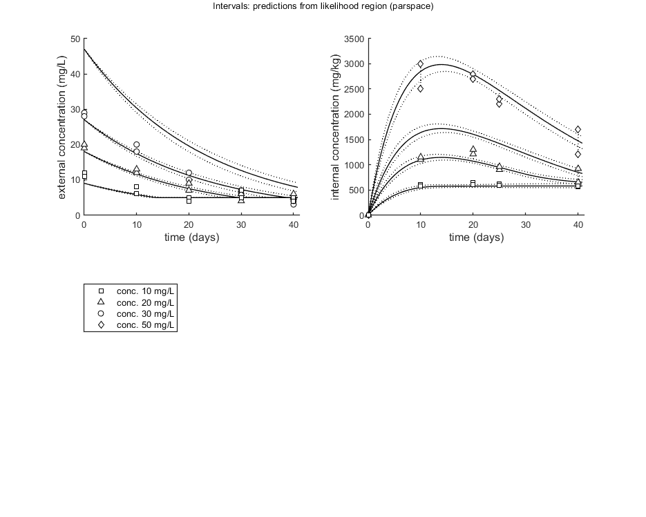
The following code can be used to make a standard plot (the same as for the fits), but with confidence intervals. Options for confidence bounds on model curves can be set using opt_conf (see prelim_checks).
Use opt_conf.type to tell calc_conf which sample to use: -1) Skips CIs (zero does the same, and an empty opt_conf as well). 1) Bayesian MCMC sample (default); CI on predictions are 95% ranges on the model curves from the sample 2) parameter sets from a joint likelihood region using the shooting method (limited sets can be used), which will yield (asymptotically) 95% CIs on predictions 3) as option 2, but using the parameter-space explorer
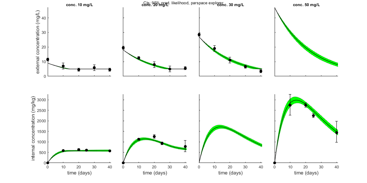
opt_conf.type    = 3; % make intervals from 1) slice sampler, 2)likelihood region shooting, 3) parspace explorer
opt_conf.lim_set = 2; % use limited set of n_lim points (1) or outer hull (2, likelihood methods only) to create CIs

out_conf = calc_conf(par_out,opt_conf); % calculate confidence intervals on model curves
calc_and_plot(par_out,opt_plot,out_conf); % call the plotting routine again to plot fits with CIs

% Here, we can also use the new plotting function for TKTD models. Even
% though this is not a TKTD model, we can still plot the internal
% concentration, with the treatments in separate panels.
glo.locC         = [1 2]; % tell plot_tktd that our first and second state variable are internal concentrations to plot
opt_tktd.repls   = 0; % plot individual replicates (1) or means (0)
opt_tktd.min     = 0; % set to 1 to show a dotted line for the control (lowest) treatment

plot_tktd(par_out,opt_tktd,opt_conf);
Amount of 0.3764 added to the chi-square criterion for inner rim
Slightly more is taken to provide a generally conservative estimate of the CIs.
Outer hull of 217 sets used.
Calculating CIs on model predictions, using sample from parspace explorer ... please be patient.
Time required: 5 mins, 30.4 secs
Plots result from the optimised parameter values.
Plot_tktd uses uses parameter set from user input for best-fit curves.
Plot_tktd uses complete parameter set from user input for best-fit curves, but CIs use all parameters from saved set.
This may lead to strange results if the input par does not result from the same fit as the saved file
(CIs may not correspond to the best curve), so interpret with care.
Amount of 0.3764 added to the chi-square criterion for inner rim
Slightly more is taken to provide a generally conservative estimate of the CIs.
Outer hull of 217 sets used.
Calculating CIs on model predictions, using sample from parspace explorer ... please be patient.
Time required: 5 mins, 33.3 secs
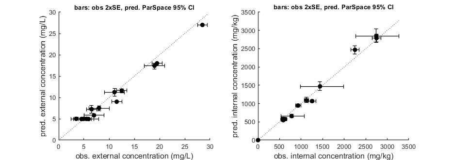
Goodness-of-fit metrics (treat with caution!)
Values below are calculated on means, incl. t=0, from the residuals
Residuals are used without accounting for any transformations
However, means are calculated with transformation (if specified in DATA)
Model efficiency (r2) NRMSE
================================================================================
body residue: 0.9716 0.1143
body residue: 0.9898 0.0851
================================================================================