BYOM, byom_bioconc_extra.m, a detailed example
- Author: Tjalling Jager
- Date: November 2021
- Web support: http://www.debtox.info/byom.html
- Back to index walkthrough_byom.html
BYOM is a General framework for simulating model systems in terms of ordinary differential equations (ODEs). The model itself needs to be specified in derivatives.m, and call_deri.m may need to be modified to the particular problem as well. The files in the engine directory are needed for fitting and plotting. Fitting relies on the multinomial likelihood for survival and independent normal distributions (if needed after transformation) for continuous data. Results are shown on screen but also saved to a log file (results.out).
In this example file (byom_bioconc_extra), we will walk step-by-step through a byom script file, explaining what happens and showing the outputs.
The model: An organism is exposed to a chemical in its surrounding medium. The animal accumulates the chemical according to standard one-compartment first-order kinetics, specified by a bioconcentration factor (Piw) and an elimination rate (ke). The chemical degrades at a certain rate (kd). When the external concentration reaches a certain concentration (Ct), degradation stops. This is useful to demonstrate the events function in call_deri.m, which catches this discontuity graciously. In the form of ODE's:
This script: byom_bioconc_extra demonstrates fitting using replicated data, with different concentration vectors in both data sets. Furthermore, several options are explained, such as the inclusion of zero-variate data and priors for Bayesian analysis. More support in the BYOM manual downloadable from here. A stripped version (less text, less options) can be found as byom_bioconc_start.m.
Copyright (c) 2012-2021, Tjalling Jager, all rights reserved.
This source code is licensed under the MIT-style license found in the
LICENSE.txt file in the root directory of BYOM.
Contents
- Initial things
- The data set
- Initial values for the state variables
- Initial values for the model parameters
- More options for the analysis
- Zero-variate data and priors for Bayesian analyses
- Time vector and labels for plots
- Calculations and plotting
- Local sensitivity analysis
- Profiling the likelihood
- Slice sampler
- Likelihood region
- Plot results with confidence intervals
- Other files: derivatives
- Other files: call_deri
Initial things
Before we start, the memory is cleared, globals are defined, and the diary is turned off (output will be collected in the file results.out). The function pathdefine.m makes sure that the engine directory is added to the path. Make sure that this script is in a directory somewhere below the BYOM folder.
clear, clear global % clear the workspace and globals
global DATA W X0mat % make the data set and initial states global variables
global glo          % allow for global parameters in structure glo
diary off           % turn off the diary function (if it is accidentaly on)
% set(0,'DefaultFigureWindowStyle','docked'); % collect all figure into one window with tab controls
set(0,'DefaultFigureWindowStyle','normal'); % separate figure windows

pathdefine(0) % set path to the BYOM/engine directory (option 1 to use parallel toolbox, if available)
glo.basenm  = mfilename; % remember the filename for THIS file for the plots
glo.saveplt = 0; % save all plots as (1) Matlab figures, (2) JPEG file or (3) PDF (see all_options.txt)
The data set
Data are entered in matrix form, time in rows, scenarios (exposure concentrations) in columns. First column are the exposure times, first row are the concentrations or scenario numbers. The number in the top left of the matrix indicates how to calculate the likelihood:
- -1 for multinomial likelihood (for survival data)
- 0 for log-transform the data, then normal likelihood
- 0.5 for square-root transform the data, then normal likelihood
- 1 for no transformation of the data, then normal likelihood
For each state variable there should be a data set in the correct position. So, DATA{1} should be the data for state variable 1, etc. The curly braces indicate that this is a 'cell array'. If there are no data for a state, use DATA{i}=0 (if you forget, this will be automatically done in the engine script prelim_checks.m). Use NaN for missing data.
Multiple data sets for each state can now be used. The first data set for state 1 becomes DATA{1,1} and the second DATA{2,1}, etc. Note that each data set is treated as completely independent. For continuous data that means that each data set has its own error distribution (either treated as 'nuisance parameter' or provided by the user in glo.var). You can enter replicated data by adding columns with the same scenario number. The scenario number should occur only once in the initial values matrix X0mat.
Note: for using survival data: enter the survival data as numbers of survivors, and not as survival probability. The model should be set up to calculate probabilities though. Therefore, the state variable is a probability, and hence the initial value in X0mat below should be a probability too (generally 1). This deluxe script automatically translates the data into probabilities for plotting the results. For survival data, the weights matrix has a different meaning: it is used to specify the number of animals that went missing or were removed during the experiment (enter the number of missing/removed animals at the time they were last seen alive in the test).
Note: In this example, the time vectors are not the same for both data sets. This is no problem for the analysis. Also the concentration vectors differ, which is also accounted for, but take care to construct the matrix with initial states carefully to catch ALL scenarios.
% observed external concentrations (two series per concentration)
DATA{1} = [ 1  10 10 20 20 30 30
            0  11 12 20 19 28 29
            10  6  8 13 12 20 18
            20  4  5  9  7 10 12
            30  5  7  6  4  6  7
            40  4  5  6  5  4  3];

% weight factors (number of replicates per observation in DATA{1})
W{1} = [10 10 10 10 10 10
        10 10 10 10 10 10
         8  8  8  8  8  9
         8  7  7  8  8  9
         6  6  6  6  6  7];

% observed internal concentrations (two series per concentration)
DATA{2} = [0.5   10  10   20   20   50   50
           0    0   0    0    0    0    0
           10 570 600 1150 1100 2500 3000
           20 610 650 1300 1210 2700 2800
           25 590 620  960  900 2300 2200
           40 580 560  920  650 1200 1700];

% if weight factors are not specified, ones are used for continuous data,
% and zero's for survival data.
Initial values for the state variables
For each state variable, we need to specify initial values for each scenario that we want to fit or simulate in the matrix X0mat. The first row specifies the scenarios (here: exposure treatments) that we want to model. Here, there are 4 scenarios in X0mat, but each data set has only 3 of them. Watch the plot to see how BYOM deals with that situation. If you do not want to fit certain scenarios (exposure treatments) from the data, simply leave them out of X0mat.
Note: if you do not want to start at t=0, specify the exact time in the global variable glo.Tinit here (e.g., glo.Tinit = 100;). If it is not specified, zero is used. The X0mat thus defines the states at glo.Tinit, and not necessarily the value at the first data point. Plotting also always starts from glo.Tinit.
Initial states, scenarios in columns, states in rows. First row are the identifiers of all scenarios (here: nominal concentrations). Second row is external concentration in mg/L, and third row body residues. For replicated data, scenarios should occur only once in X0mat.
X0mat = [10 20 30 50    % the scenarios (here nominal concentrations)
          9 18 27 47    % initial values state 1 (actual external concentrations)
          0  0  0  0];  % initial values state 2 (internal concentrations)

% Note: The initial external concentrations are slightly different from
% the "nominal" ones.

% X0mat(:,3) = []; % for example, quickly remove the third scenario (conc 30)
Initial values for the model parameters
Model parameters are part of a 'structure' for easy reference. This means that you can address parameters by their name, instead of their position in a parameter vector. This makes the model definition in derivatives.m a lot easier. For each parameter, provide the initial value, whether you want to fit it or fix it to the initial value, the minimum bound, the maximum bound, and whether to fit the parameter on log10-scale or on normal scale. Fitting on log-scale is advisable for parameters that can span a very wide range; the optimisation routine can search this range more effectively if it is on log-scale. If you do not include this last value, a one will be filled in by prelim_checks.m (which means fitting on normal scale).
% syntax: par.name = [startvalue fit(0/1) minval maxval optional:log/normal scale (0/1)];
par.kd    = [0.1  1 1e-3 10  1];  % degradation rate constant, d-1
par.ke    = [0.2  1 1e-3 10  1];  % elimination rate constant, d-1
par.Piw   = [200  1 100  1e3 1];  % bioconcentration factor, L/kg
par.Ct    = [5    0 0    10  1];  % threshold external concentration where degradation stops, mg/L

% % Optionally, include an initial state as parameter (requires changes in call_deri.m too)
% par.Ci0   = [100  0 0 1e6];  % initial internal concentration (mg/L)
More options for the analysis
Optionally, global parameters can be used in the structure glo (not fitted). However, see the text file reserved_globals.txt for names to avoid.
% % specify globals for parameters that are never fitted
% glo.Ct = 5; % the threshold could be made into a fixed global (also modify derivatives.m)
% % Special globals to modify the optimisation (used in transfer.m)
% glo.wts = [1 10];  % different weights for different data sets (same size as DATA)
% glo.var = [10 20]; % supply residual variance for each data set, after transformation (same size as DATA)
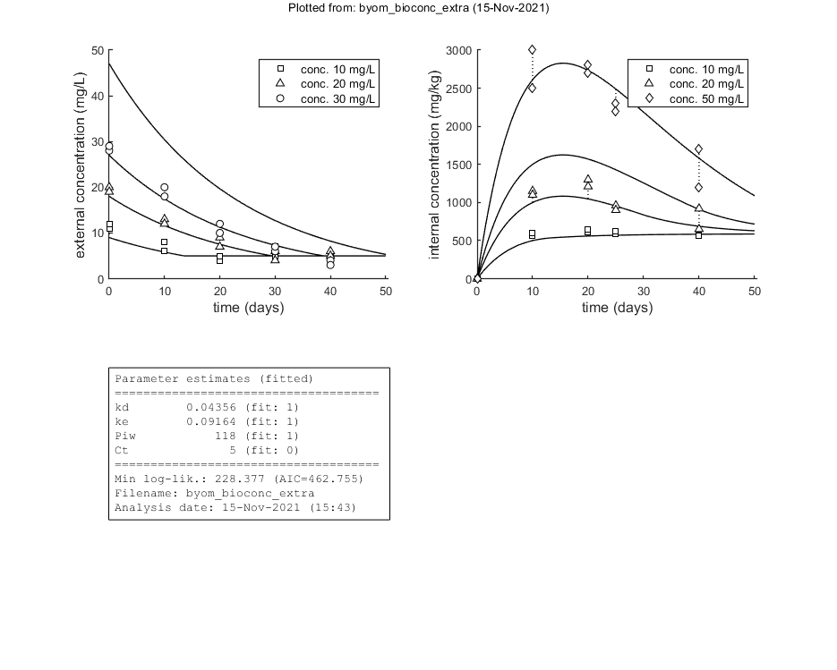
Zero-variate data and priors for Bayesian analyses
Optionally, zero-variate data can be included. The corresponding model value needs to be calculated in call_deri.m, so modify that file too! You can make up your own parameter names in the structure zvd. Optionally, prior distributions can be specified for parameters, see the file calc_prior.m for the definition of the distributions. You must use the exact same names for the prior parameters as used in the par structure. If you do not specify zvd and/or pri in your scripts, these options are simply not used in the analysis.
Note: the priors are also used for 'frequentist' analysis. They are treated as independent additional likelihood functions.
zvd.ku = [10 0.5]; % example zero-variate data point for uptake rate, with normal s.d.

% First element in pri is the choice of distribution.
pri.Piw   = [2 116 121 118]; % triangular with min, max and center
pri.ke    = [3 0.2 0.1];     % normal with mean and sd
% If no prior is defined, the min-max bounds will define a uniform one.
% Note that the prior is always defined on normal scale, also when the
% parameter will be fitted on log scale.
Time vector and labels for plots
Specify what to plot. This also involves the time vector for the model lines (which may be taken differently than the time vector in the data set). If time vector glo.t is not specified, a default is constructed, based on the data set. You can specify the text that you would like to use for the axes, and the text used for the legend (which always includes the identifier for the scenario: the values in the first row of X0mat).
glo.t = linspace(0,50,100); % time vector for the model curves in days

% specify the y-axis labels for each state variable
glo.ylab{1} = 'external concentration (mg/L)';
glo.ylab{2} = 'internal concentration (mg/kg)';
% specify the x-axis label (same for all states)
glo.xlab    = 'time (days)';
glo.leglab1 = 'conc. '; % legend label before the 'scenario' number
glo.leglab2 = 'mg/L'; % legend label after the 'scenario' number

prelim_checks % script to perform some preliminary checks and set things up
% Note: prelim_checks also fills all the options (opt_...) with defauls, so
% modify options after this call, if needed.
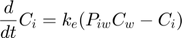
Calculations and plotting
Here, the functions are called that will do the calculation and the plotting. Note that calc_plot can provide all of the plotting information as output, so you can also make your own customised plots. This section, by default, makes a multiplot with all state variables (each in its own panel of the multiplot). When the model is fitted to data, output is provided on the screen (and added to the log-file results.out). The zero-variate data point is also plotted with its prediction (although the legend obscures it here).
Options for the plotting can be set using opt_plot (see prelim_checks.m). Options for the optimisation routine can be set using opt_optim. Options for the ODE solver are part of the global glo.
You can turn on the events function there too, to smoothly catch the discontinuity in the model. For the demo, the iterations were turned off (opt_optim.it = 0).
glo.eventson   = 1; % events function on (1) or off (0)
glo.useode     = 1; % calculate model using ODE solver (1) or analytical solution (0)
opt_optim.it   = 0; % show iterations of the optimisation (1, default) or not (0)
opt_plot.annot = 1; % extra subplot in multiplot for fits: 1) box with parameter estimates, 2) overall legend
opt_plot.bw    = 1; % if set to 1, plots in black and white with different plot symbols

% glo.diary = 'test_results.out'; % use a different name for the diary

% optimise and plot (fitted parameters in par_out)
par_out = calc_optim(par,opt_optim); % start the optimisation
calc_and_plot(par_out,opt_plot);     % calculate model lines and plot them

% save_plot(gcf,'fit_example',[],3) % save active figure as PDF (see save_plot for more options)

% return % stop here, and run analyses below manually later
Goodness-of-fit measures for each state and each data set (R-square)
Based on the individual replicates, accounting for transformations, and including t=0
state 1. 0.96
state 2. 0.99
=================================================================================
Results of the parameter estimation with BYOM version 6.0 BETA 6
=================================================================================
Filename : byom_bioconc_extra
Analysis date : 15-Nov-2021 (15:43)
Data entered :
data state 1: 5x6, continuous data, no transf.
data state 2: 5x6, continuous data, power 0.50 transf.
Search method: Nelder-Mead simplex direct search, 2 rounds.
The optimisation routine has converged to a solution
Total 150 simplex iterations used to optimise.
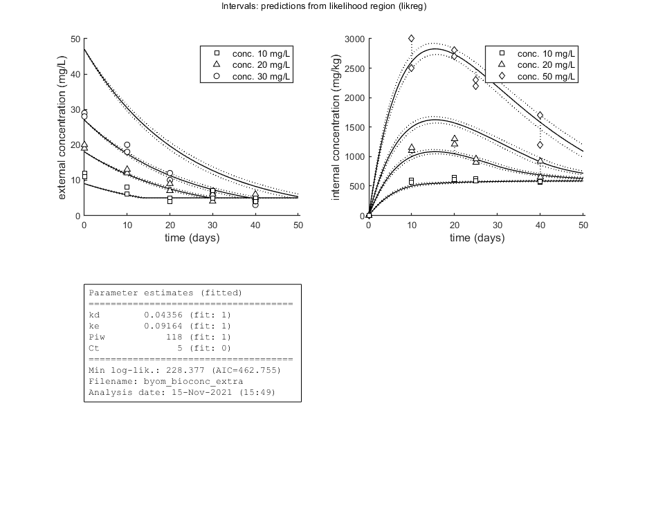
Minus log-likelihood has reached the value 228.38 (AIC=462.75).
=================================================================================
kd 0.04356 (fit: 1, initial: 0.1) prior: unif (0.001-10)
ke 0.09164 (fit: 1, initial: 0.2) prior: norm (mn 0.2,sd 0.1)
Piw 118.0 (fit: 1, initial: 200) prior: tri (116-118-121)
Ct 5 (fit: 0, initial: 5) prior: unif (0-10)
=================================================================================
Final values for zero-variate data points included:
ku 10.81 (data point: 10, sd: 0.5)
=================================================================================
Time required: 2.1 secs
Plots result from the optimised parameter values.
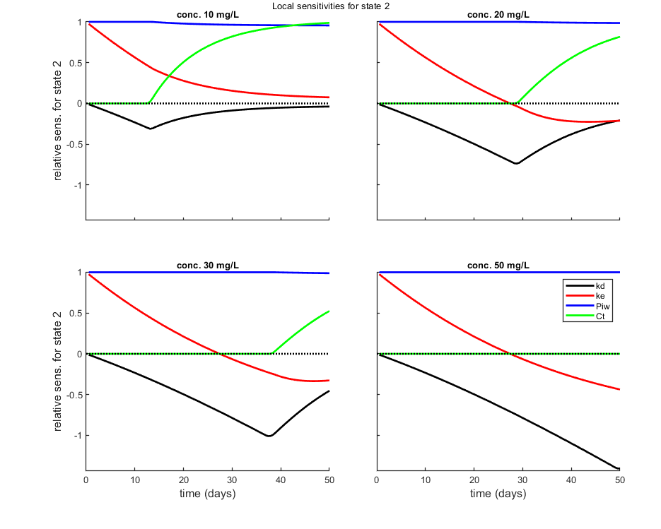
Local sensitivity analysis
Local sensitivity analysis of the model. All model parameters are increased one-by-one by a small percentage. The sensitivity score is by default scaled (dX/X p/dp) or alternatively absolute (dX p/dp).
Options for the sensitivity can be set using opt_sense (see prelim_checks.m).
% UNCOMMENT LINE(S) TO CALCULATE
opt_sens.state = 2; % vector with state variables for the sensitivity analysis (0 does all, if sens>0)
calc_localsens(par_out,opt_sens)
Profiling the likelihood
By profiling you make robust confidence intervals for one or more of your parameters. Use the names of the parameters as they occurs in your parameter structure par above. This can be a single string (e.g., 'kd'), a cell array of strings (e.g., {'kd','ke'}), or 'all' to profile all fitted parameters. This example produces a profile for each parameter and provides the 95% confidence interval (on screen and indicated by the horizontal broken line in the plot).
Notes: profiling for complex models is a slow process, so grab a coffee! If the profile finds a better solution, it breaks the analysis (as long as you keep the default opt_prof.brkprof=1) and displays the parameters for the new optimum on screen (and in results.out). For the NON-parallel version of calc_proflik, the new optimum is also immediately saves to the log file profiles_newopt.out. You can break of the analysis by pressing ctrl-c anytime, and use the values from the log file to restart (copy the better values into your par structure). For parallel processing, saving would need more thought.
Options for profiling can be set using opt_prof (see prelim_checks.m).
opt_prof.detail   = 1; % detailed (1) or a coarse (2) calculation
opt_prof.subopt   = 0; % number of sub-optimisations to perform to increase robustness
opt_prof.brkprof  = 2; % when a better optimum is located, stop (1) or automatically refit (2)

% UNCOMMENT LINE(S) TO CALCULATE
par_better = calc_proflik(par_out,'all',opt_prof,opt_optim);  % calculate a profile
if ~isempty(par_better)                 % if the profiling found a better optimum ...
    print_par(par_better) % display on screen in formatted manner, so it can be copied into the code
    calc_and_plot(par_better,opt_plot); % calculate model lines and plot them
end
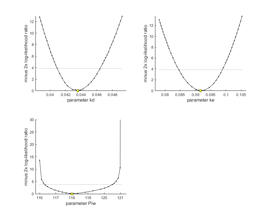
95% confidence interval(s) from the profile(s)
=================================================================================
kd         interval:    0.04093 -  0.04641
ke         interval:    0.08457 -  0.09880
Piw        interval:      116.3 -  120.5
=================================================================================

Time required: 1 min, 55.1 secs
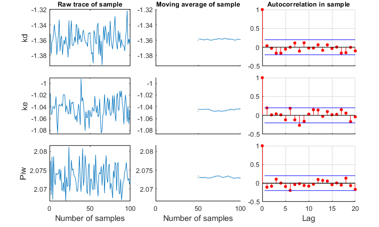
Slice sampler
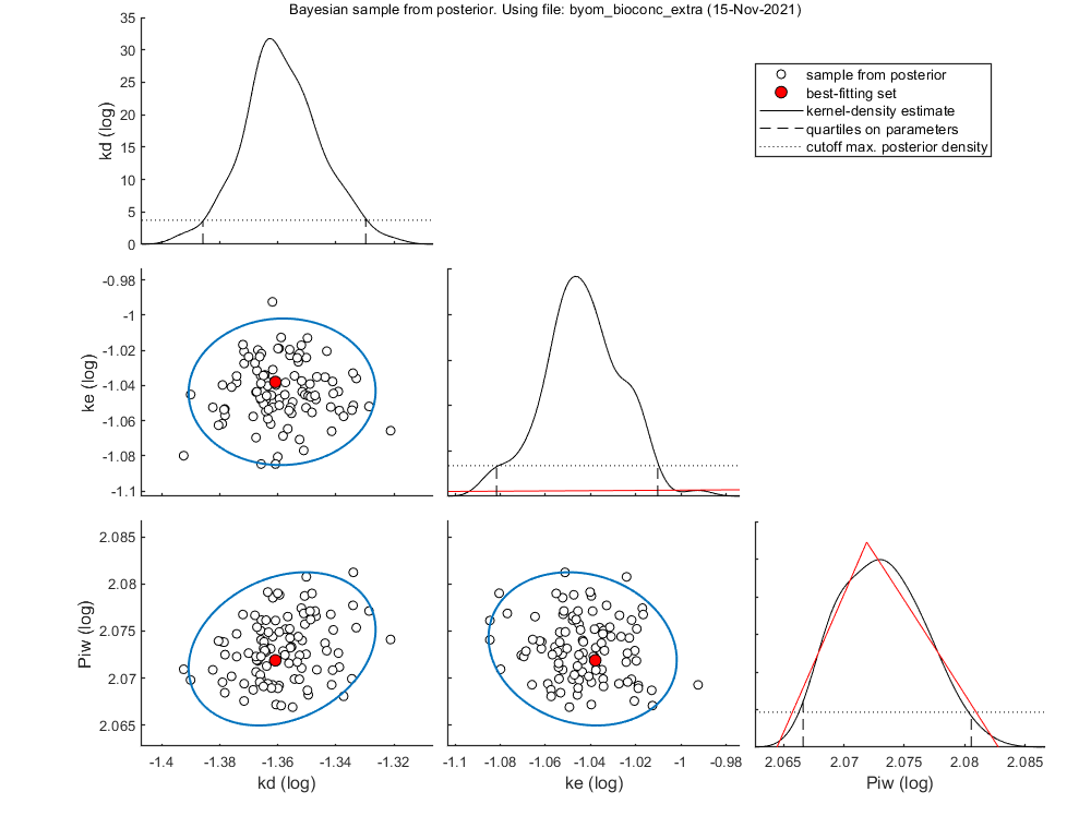
The slice sampler can be used for a Bayesian analysis as it provides a sample from the posterior distribution. A .mat file is saved which contains the sample, to use later for e.g., intervals on model predictions. The output includes the Markov chain and marginal distributions for each fitted parameter. The function calc_conf can be used to put confidence intervals on the model lines.
Notes: MCMC is also slow process for complex models, so consider another coffee! If a prior is specified, it is plotted in the marginal posterior plot as a red distribution. Two types of credible intervals are generated:
- Highest probability regions. This captures the 95% of the parameter values with the highest posterior probability. it is calculated by lowering the horizotal dotted line in the figures for each parameters, until the area between the cut-off points captures 95% of the density. This can lead to unequal probabilities in the tails.
- Quantiles. The region between the 2.5 and 97.5% quantiles is taken. This leads to 2.5% probability in each tail. This is shown in the plots by the broken vertical lines.
Options for the slice sampling can be set using opt_slice (see prelim_checks.m). Options for confidence bounds on model curves can be set in opt_conf (see prelim_checks).
Taking on parameters on log scale helps, as the slice sampler seems quite bad at obtaining a representative sample when the parameters have very different ranges. Thinning will be needed to reduce the autocorrelation (which is too much here). Note the plot that is produced with details of the sample!
% UNCOMMENT LINE(S) TO CALCULATE
opt_slice.thin     = 10; % thinning of the sample (keep one in every 'thin' samples)
opt_slice.burn     = 100; % number of burn-in samples (0 is no burn in)
opt_slice.alllog   = 1; % set to 1 to put all parameters on log-scale before taking the sample
calc_slice(par_out,100,opt_slice); % second argument number of samples (-1 to re-use saved sample from previous runs)
Calculating sample from posterior density ... please be patient.
Median and credible intervals (95% highest posterior density, 2.5-97.5% quantiles)
======================================================================================
kd            0.04367 hdr:     0.0412 -    0.04685 quant:    0.04113 -     0.0468
ke             0.0902 hdr:     0.0829 -    0.09777 quant:    0.08287 -    0.09767
Piw             118.3 hdr:      116.5 -      120.3 quant:      116.6 -      120.4
======================================================================================

Correlation matrix from the MCMC sample
======================================================================================
               kd          ke         Piw
kd              1
ke        0.01372           1
Piw          0.25     -0.1477           1
Note: some parameters have been estimated on log-scale; correlations are also on log-scale for these parameters.
======================================================================================

Number of MCMC samples taken: 100
Time required: 3 mins, 47.9 secs
Likelihood region
Another way to make intervals on model predictions is to use a sample of parameter sets taken from the joint likelihood-based conf. region. This is done by the function calc_likregion.m. It first does profiling of all fitted parameters to find the edges of the region. Then, Latin-Hypercube shooting, keeping only those parameter combinations that are not rejected at the 95% level in a lik.-rat. test. The inner rim will be used for CIs on forward predictions.
Options for the likelihood region can be set using opt_likreg (see prelim_checks.m). For the profiling part, use the options in opt_prof.
opt_prof.detail  = 1; % detailed (1) or a coarse (2) calculation
opt_prof.subopt  = 0; % number of sub-optimisations to perform to increase robustness
opt_prof.re_fit  = 1; % set to 1 to automatically refit when a new optimum is found
opt_likreg.skipprof = 0; % skip profiling step; use boundaries from saved likreg set (1) or profiling (2)

par_better = calc_likregion(par_out,500,opt_likreg,opt_prof,opt_optim);
% Second entry is the number of accepted parameter sets to aim for. Use -1
% here to use a saved set.

if isstruct(par_better) % if the profiling found a better optimum ...
    print_par(par_better) % display on screen in formatted manner, so it can be copied into the code
    calc_and_plot(par_better,opt_plot); % calculate model lines and plot them
    return % stop here, and don't go into plotting with CIs
end
Calculating profiles and sample from confidence region ... please be patient.

95% confidence interval(s) from the profile(s)
=================================================================================
kd         interval:    0.04093 -  0.04641
ke         interval:    0.08457 -  0.09880
Piw        interval:      116.3 -  120.5
=================================================================================

Time required: 5 mins, 37.1 secs

Starting with obtaining a sample from the joint confidence region.
Bursts of 100 samples, until at least 500 samples are accepted in inner rim.
Total number of parameters tried (profile points have been added): 3490
of which accepted in the conf. region: 1521, and in inner rim: 563
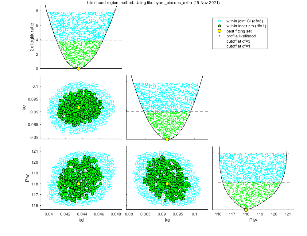
Time required: 6 mins, 10.4 secs
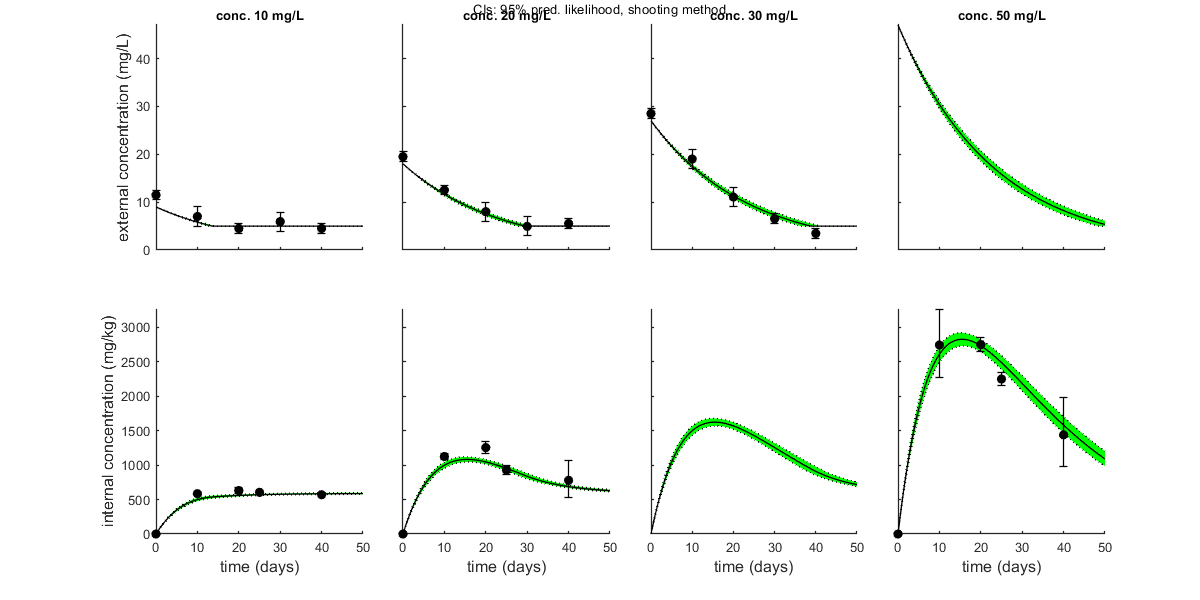
Plot results with confidence intervals
The following code can be used to make a standard plot (the same as for the fits), but with confidence intervals. Options for confidence bounds on model curves can be set using opt_conf (see prelim_checks).
Use opt_conf.type to tell calc_conf which sample to use: -1) Skips CIs (zero does the same, and an empty opt_conf as well). 1) Bayesian MCMC sample (default); CI on predictions are 95% ranges on the model curves from the sample 2) parameter sets from a joint likelihood region using the shooting method (limited sets can be used), which will yield (asymptotically) 95% CIs on predictions 3) as option 2, but using the parameter-space explorer
opt_conf.type    = 2; % make intervals from 1) slice sampler, 2) likelihood region shooting, 3) parspace explorer
opt_conf.lim_set = 2; % use limited set of n_lim points (1) or outer hull (2, likelihood methods only) to create CIs
opt_conf.sens    = 0; % type of analysis 0) no sensitivities 1) corr. with state, 2) corr. with state/control, 3) corr. with relative change of state over time

out_conf = calc_conf(par_out,opt_conf);   % calculate confidence intervals on model curves
calc_and_plot(par_out,opt_plot,out_conf); % call the plotting routine again to plot fits with CIs

% Here, we can also use the new plotting function for TKTD models. Even
% though this is not a TKTD model, we can still plot the internal
% concentration, with the treatments in separate panels.
glo.locC       = [1 2]; % tell plot_tktd that our first and second state variable are internal concentrations to plot
opt_tktd.repls = 0;     % plot individual replicates (1) or means (0)
opt_tktd.min   = 0;     % set to 1 to show a dotted line for the control (lowest) treatment

plot_tktd(par_out,opt_tktd,opt_conf);
Amount of 0.3764 added to the chi-square criterion for inner rim
Slightly more is taken to provide a generally conservative estimate of the CIs.
Outer hull of 237 sets used.
Calculating CIs on model predictions, using sample from joint likelihood region ... please be patient.
Time required: 6 mins, 13.5 secs
Plots result from the optimised parameter values.
Plot_tktd uses uses parameter set from user input for best-fit curves.
Plot_tktd uses complete parameter set from user input for best-fit curves, but CIs use all parameters from saved set.
This may lead to strange results if the input par does not result from the same fit as the saved file
(CIs may not correspond to the best curve), so interpret with care.
Amount of 0.3764 added to the chi-square criterion for inner rim
Slightly more is taken to provide a generally conservative estimate of the CIs.
Outer hull of 237 sets used.
Calculating CIs on model predictions, using sample from joint likelihood region ... please be patient.
Time required: 6 mins, 16.9 secs
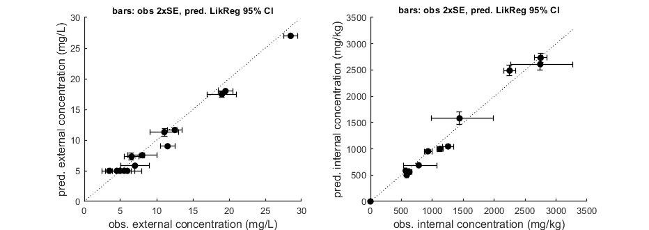
Goodness-of-fit metrics (treat with caution!)
Values below are calculated on means, incl. t=0, from the residuals
Residuals are used without accounting for any transformations
However, means are calculated with transformation (if specified in DATA)
Model efficiency (r2) NRMSE
================================================================================
body residue: 0.9719 0.1138
body residue: 0.9848 0.1039
================================================================================
Other files: derivatives
To archive analyses, publishing them with Matlab is convenient. To keep track of what was done, the file derivatives.m can be included in the published result.
%% BYOM function derivatives.m (the model in ODEs)
%
%  Syntax: dX = derivatives(t,X,par,c,glo)
%
% This function calculates the derivatives for the model system. It is
% linked to the script files <byom_bioconc_extra.html byom_bioconc_extra.m>
% and <byom_bioconc_start.html byom_bioconc_start.m>. As input,
% it gets:
%
% * _t_   is the time point, provided by the ODE solver
% * _X_   is a vector with the previous value of the states
% * _par_ is the parameter structure
% * _c_   is the external concentration (or scenario number)
% * _glo_ is the structure with information (normally global)
%
% Note: _glo_ is now an input to this function rather than a global. This
% makes the code considerably faster.
%
% Time _t_ and scenario name _c_ are handed over as single numbers by
% <call_deri.html call_deri.m> (you do not have to use them in this
% function). Output _dX_ (as vector) provides the differentials for each
% state at _t_.
%
% * Author: Tjalling Jager
% * Date: November 2021
% * Web support: <http://www.debtox.info/byom.html>
% * Back to index <walkthrough_byom.html>
%
%  Copyright (c) 2012-2021, Tjalling Jager, all rights reserved.
%  This source code is licensed under the MIT-style license found in the
%  LICENSE.txt file in the root directory of BYOM.

%% Start
% Note that, in this example, variable _c_ (the scenario identifier) is not
% used in this function. The treatments differ in their initial exposure
% concentration that is set in X0mat. Also, the time _t_ and structure _glo_ are not
% used here.

function dX = derivatives(t,X,par,c,glo)

%% Unpack states
% The state variables enter this function in the vector _X_. Here, we give
% them a more handy name.

Cw = X(1); % state 1 is the external concentration
Ci = X(2); % state 2 is the internal concentration

%% Unpack parameters
% The parameters enter this function in the structure _par_. The names in
% the structure are the same as those defined in the byom script file. The
% 1 between parentheses is needed for fitting the model, as each parameter
% has 4-5 associated values.

kd   = par.kd(1);   % degradation rate constant, d-1
ke   = par.ke(1);   % elimination rate constant, d-1
Piw  = par.Piw(1);  % bioconcentration factor, L/kg
Ct   = par.Ct(1);   % threshold external concentration that stops degradation, mg/L

% % Optionally, include the threshold concentration as a global (see script)
% Ct   = glo.Ct;      % threshold external concentration that stops degradation, mg/L

%% Calculate the derivatives
% This is the actual model, specified as a system of two ODEs:
%
% $$ \frac{d}{dt}C_w=-k_d C_w \quad \textrm{as long as } C_w>C_t $$
%
% $$ \frac{d}{dt}C_i=k_e(P_{iw}C_w-C_i) $$

if Cw > Ct          % if we are above the critical internal concentration ...
    dCw = -kd * Cw; % let the external concentration degrade
else                % otherwise ...
    dCw = 0;        % make the change in external concentration zero
end

dCi = ke * (Piw * Cw - Ci); % first order bioconcentration

dX = [dCw;dCi]; % collect both derivatives in one vector dX
Other files: call_deri
To archive analyses, publishing them with Matlab is convenient. To keep track of what was done, the file call_deri.m can be included in the published result.
%% BYOM function call_deri.m (calculates the model output)
%
%  Syntax: [Xout,TE,Xout2,zvd] = call_deri(t,par,X0v,glo)
%
% This function calls the ODE solver to solve the system of differential
% equations specified in <derivatives.html derivatives.m>, or the explicit
% function(s) in <simplefun.html simplefun.m>. As input, it gets:
%
% * _t_   the time vector
% * _par_ the parameter structure
% * _X0v_ a vector with initial states and one concentration (scenario number)
% * _glo_ the structure with various types of information (used to be global)
%
% The output _Xout_ provides a matrix with time in rows, and states in
% columns. This function calls <derivatives.html derivatives.m>. The
% optional output _TE_ is the time at which an event takes place (specified
% using the events function). The events function is set up to catch
% discontinuities. It should be specified according to the problem you are
% simulating. If you want to use parameters that are (or influence) initial
% states, they have to be included in this function. Optional output Xout2
% is for additional uni-variate data (not used here), and zvd is for
% zero-variate data (used in <byom_bioconc_extra.html
% byom_bioconc_extra.m>).
%
% * Author: Tjalling Jager
% * Date: November 2021
% * Web support: <http://www.debtox.info/byom.html>
% * Back to index <walkthrough_byom.html>
%
%  Copyright (c) 2012-2021, Tjalling Jager, all rights reserved.
%  This source code is licensed under the MIT-style license found in the
%  LICENSE.txt file in the root directory of BYOM.

%% Start

function [Xout,TE,Xout2,zvd] = call_deri(t,par,X0v,glo)

% initialise extra outputs as empty for when they are not used
Xout2    = []; % additional uni-variate output
zvd      = []; % additional zero-variate output

% Note: if these options are not used, these variables must be defined as
% empty as they are outputs of this function.

% if needed, calculate model values for zero-variate data from parameter
% set; these lines can be removed if no zero-variate data are used
if ~isempty(glo.zvd) % if there are zero-variate data defined (see byom_bioconc_extra)
    zvd       = glo.zvd; % copy zero-variate data structure to zvd
    zvd.ku(3) = par.Piw(1) * par.ke(1); % add model prediction as third value in zvd
else % if there are no zero-variate data defined (as in byom_bioconc_start)
    zvd       = []; % additional zero-variate output, output defined as empty matrix
end

%% Initial settings
% This part extracts optional settings for the ODE solver that can be set
% in the main script (defaults are set in prelim_checks). The useode option
% decides whether to calculate the model results using the ODEs in
% <derivatives.html derivatives.m>, or the analytical solution in
% <simplefun.html simplefun.m>. Using eventson=1 turns on the events
% handling. Also modify the sub-function at the bottom of this function!
% Further in this section, initial values can be determined by a parameter
% (overwrite parts of X0), and zero-variate data can be calculated. See the
% example BYOM files for more information.

useode   = glo.useode; % calculate model using ODE solver (1) or analytical solution (0)
eventson = glo.eventson; % events function on (1) or off (0)
stiff    = glo.stiff; % set to 1 or 2 to use a stiff solver instead of the standard one

% Unpack the vector X0v, which is X0mat for one scenario
X0 = X0v(2:end); % these are the intitial states for a scenario
% % if needed, extract parameters from par that influence initial states in X0
% Ci0   = par.Ci0(1); % example: parameter for the internal concentration
% X0(2) = Ci0; % put this parameter in the correct location of the initial vector

%% Calculations
% This part calls the ODE solver (or the explicit model in <simplefun.html
% simplefun.m>) to calculate the output (the value of the state variables
% over time). There is generally no need to modify this part. The solver
% ode45 generally works well. For stiff problems, the solver might become
% very slow; you can try ode15s instead.

c  = X0v(1);     % the concentration (or scenario number)
t  = t(:);       % force t to be a row vector (needed when useode=0)

TE = 0; % dummy for time of events

if useode == 1 % use the ODE solver to calculate the solution
    % Note: set options AFTER the 'if useode == 1' as odeset takes
    % considerable calculation time, which is not needed when using the
    % analytical solution. Also note that the global _glo_ is now input to
    % the derivatives function. This increases calculation speed.

    % specify options for the ODE solver; feel free to change the
    % tolerances, if you know what you're doing (for some problems, it is
    % better to set them much tighter, e.g., both to 1e-9)
    reltol = 1e-4;
    abstol = 1e-7;
    options = odeset; % start with default options
    if eventson == 1
        options = odeset(options,'Events',@eventsfun,'RelTol',reltol,'AbsTol',abstol); % add an events function and tigher tolerances
    else
        options = odeset(options,'RelTol',reltol,'AbsTol',abstol); % only specify tightened tolerances
    end
    % options = odeset(options,'InitialStep',max(t)/1000,'MaxStep',max(t)/100); % specify smaller stepsize

    % call the ODE solver (try ode15s for stiff problems, and possibly with for pulsed forcings)
    if isempty(options.Events) % if no events function is specified ...
        switch stiff
            case 0
                [~,Xout] = ode45(@derivatives,t,X0,options,par,c,glo);
            case 1
                [~,Xout] = ode113(@derivatives,t,X0,options,par,c,glo);
            case 2
                [~,Xout] = ode15s(@derivatives,t,X0,options,par,c,glo);
        end
    else % with an events functions ... additional output arguments for events:
        % TE catches the time of an event, YE the states at the event, and IE the number of the event
        switch stiff
            case 0
                [~,Xout,TE,YE,IE] = ode45(@derivatives,t,X0,options,par,c,glo);
            case 1
                [~,Xout,TE,YE,IE] = ode113(@derivatives,t,X0,options,par,c,glo);
            case 2
                [~,Xout,TE,YE,IE] = ode15s(@derivatives,t,X0,options,par,c,glo);
        end
    end
else % alternatively, use an explicit function provided in simplefun
    Xout = simplefun(t,X0,par,c,glo);
end

if isempty(TE) || all(TE == 0) % if there is no event caught
    TE = +inf; % return infinity
end

%% Output mapping
% _Xout_ contains a row for each state variable. It can be mapped to the
% data. If you need to transform the model values to match the data, do it
% here.

% Xout(:,1) = Xout(:,1).^3; % e.g., do something on first column, like cube it ...

% % To obtain the output of the derivatives at each time point. The values in
% % dXout might be used to replace values in Xout, if the data to be fitted
% % are the changes (rates) instead of the state variable itself.
% % dXout = zeros(size(Xout)); % initialise with zeros
% for i = 1:length(t) % run through all time points
%     dXout(i,:) = derivatives(t(i),Xout(i,:),par,c,glo);
%     % derivatives for each stage at each time
% end

%% Events function
% Modify this part of the code if _eventson_=1. This subfunction catches
% the 'events': in this case, it looks for the external concentration where
% degradation stops. This function should be adapted to the problem you are
% modelling (this one matches the byom_bioconc_... files). You can catch
% more events by making a vector out of _values_.
%
% Note that the eventsfun has the same inputs, in the same sequence, as
% <derivatives.html derivatives.m>.

function [value,isterminal,direction] = eventsfun(t,X,par,c,glo)

Ct      = par.Ct(1); % threshold external concentration where degradation stops
nevents = 1;         % number of events that we try to catch

value       = zeros(nevents,1); % initialise with zeros
value(1)    = X(1) - Ct;        % thing to follow is external concentration (state 1) minus threshold
isterminal  = zeros(nevents,1); % do NOT stop the solver at an event
direction   = zeros(nevents,1); % catch ALL zero crossing when function is increasing or decreasing