Getting started with BYOM
Back to the overview of the manual
Contents
Installation
To install BYOM, unpack the ZIP file to a location of your choice. Do not rename any of the directories. The first files to study are in the examples directory. It is best not to modify these files, so you can always return to a working model. To create your own model, copy the files in examples to a new directory, somewhere as sub- or sub-sub-directory of the BYOM directory (do not rename the BYOM directory, put all new directories below this one, and don't start any of the directory names with BYOM.
Make sure that the new directory includes a copy of the functions derivatives.m (which holds your model equations), call_deri.m (calls the derivatives functions with initial state values and includes the events function), and pathdefine.m (this makes sure the correct engine directories such as ../BYOM/engine are added to the Matlab path). Modify derivatives.m to represent your own models. In several cases, (slight) modifications of call_deri.m will be needed. There is no need to change the functions in the engine folders, and in general I would advise to leave them alone unless you REALLY know what you're doing.
I suggest naming your script files starting with byom_ to clearly distinguish them from the functions. Do not include spaces in script or directory names (Matlab does not like that). The engine directories contains the files for fitting the model to data; there should be no need to modify these files.
The example in this manual
To explain how BYOM works, I am first running through a very simple example. This example concerns biocontration with the standard one-compartment model. The internal concentration (Ci) is given by this ODE:
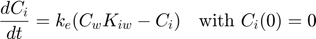
Here, Cw is the external concentration in water, Kiw is the partition coefficient between water and the organism (the bioconcentration factor), and ke is the elimination rate.
We are going to fit this model to a data set from Gomez et al. (2012), http://dx.doi.org/10.1007/s11356-012-0964-3 on accumulation of two exposure levels of tetrazepam in the mussel Mytilus galloprovincialis. Seven days of exposure exposure is followed by seven days of depuration in clean water. The same data set was used for the modelling chapter in the Marine Ecotoxicology textbook, but here we use the means rather than the individual replicates (see notes at the end of this page for comments on the statistics).
First, I will go through the the important elements of BYOM in isolation, and then show what it looks like in the BYOM script.
lets_get_started
What you need to put in
Entering data. The data are entered in the main script in a cell array, like so:
% Internal concentration in mussels in ug/kg dwt, time in days, exposure
% concentrations in ug/L.
DATA{1} = [1           2.3         14.5
            0            0            0
            1       52.542        634.1
            3       92.128       917.68
            7       192.17       1438.8
            8       71.975       783.81
           10       33.108       356.28
           14       6.4778       128.48];
The structure DATA holds all of your data in a specific format. In BYOM data sets are always linked to state variables. Our model has only one state (the internal concentration Ci), so we place our data set in location one in the cell array (hence DATA{1}). If the model has more state variables, you can add additional data sets as DATA{2} etc. As DATA is a cell array, the different data sets do not need to have the same size. If you have no data for a state, leave it out or just set it to zero.
The first element of the data matrix (top left) is for a flag how to treat the data. The 1 implies that it is continuous data, and that we don't want to use data transformation. The optimisation criterion is derived from the normal likelihood function, and thus assumes independent normal distributions, with constant variance, for the residuals. In this simple case, this approach is fully equivalent to least squares.
The other elements of the top row are the identifiers for the two exposure scenarios; in this case, the external concentrations in water during the exposure phase. These numbers are handed over to call_deri and derivatives as the variable c, and they are used for the legends in the plots. Below the top row are the time vector (in the first column) and the observations.
When we ask Matlab what the data is, we see that it is a cell array, containing a single cell, which in turn contains an 8x3 matrix with numbers:
DATA
DATA =

  1×1 cell array

    {8×3 double}
Note that a data set may contain duplicate time points, and duplicate exposure treatments; no problem.
Initial values. Every state values needs to have initial values (the value at t=0) for each of the scenarios we like to run. These are the same identifiers c as we used in the data set. In BYOM, this is taken care of by the matrix X0mat:
X0mat = [2.3 14.5  % the scenarios (here exposure concentrations)
         0  0  ];  % initial values state 1 (internal concentrations)
This tells BYOM that we want to run two scenarios (the two we also identified in DATA), and that the initial internal concentration is zero in both treatments. Note that X0mat may contain less scenarios than the data, or more. Only the scenarios in X0mat will be run, and the corresponding model curves plotted. If there is any data for these scenarios, they will be used for fitting and shown in the plots. If not, only a simulation is provided.
Specifying parameters. In BYOM, model parameters are part of a structure. This is very useful, as we can address them in derivatives and elsewhere by a name, which reduces the chance of errors. In your main script, you need to specify the parameters, provide them with a starting value, tell BYOM whether it needs to fit the parameter or fix it, and provide min-max bounds:
% syntax: par.name = [startvalue fit(0/1) minval maxval];
par.Kiw   = [50   1    0 1e6];  % bioconcentration factor, L/kg
par.ke    = [0.2  1 1e-3 100];  % elimination rate constant, d-1
We use wide min-max bounds in this case. For rate constants, like ke, it is generally a good idea to make sure they do not run off to zero or infinity (that can lead to numerical issues such as extreme slowness of the calculations).
The nice thing about using a structure is that we can refer to parameters by their name, instead of its position in a vector. When we ask what par looks like after this:
par
par =

  struct with fields:

    Kiw: [50 1 0 1000000]
     ke: [0.2000 1 1.0000e-03 100]
And we can also ask for a specific parameter by using its name:
par.ke
ans =

    0.2000    1.0000    0.0010  100.0000
Settings for modelling and plotting. BYOM will choose its own time vector, based on the time points in your data sets. What I do need to specify is what text I would like to see with the axes of my plots:
% specify the y-axis labels for each state variable
glo.ylab{1} = ['internal concentration (',char(181),'g/kg dwt)'];
% specify the x-axis label (same for all states)
glo.xlab    = 'time (days)';
The specification of the y-label is a cell (hence the {1}). This is handy as each state can have its own y-axis label. There is only one x-label, which is usually time. The char(181) is a way to get the micro symbol for the units in there.
Next, specify what you would like to do with the legends. The scenarios (the first row in X0mat) will always be part of the legend, but there can be some text in front and after it:
glo.leglab1 = 'conc. '; % legend label before the 'scenario' number
glo.leglab2 = [char(181),'g/L']; % legend label after the 'scenario' number
This will give us a nice legend when we're plotting. Now, let's look what the global variable glo now contains:
glo
glo =

  struct with fields:

       ylab: {'internal concentration (µg/kg dwt)'}
       xlab: 'time (days)'
    leglab1: 'conc. '
    leglab2: 'µg/L'
The model. All of the information above had to be entered in the main script. The model, however, goes in the file derivatives.m. There, you first need to unpack the parameters from their structure (that leads to a more readable code):
Kiw  = par.Kiw(1);  % bioconcentration factor, L/kg
ke   = par.ke(1);   % elimination rate constant, d-1
Note that I only want to know the first element of the parameter vector; its value. The other information is used elsewhere in the model, and we don't have to care about that.
The scenario (the first rows X0mat) enters derivatives through the variable c. In this case, our scenario identifiers are the concentration in the exposure phase, so that makes our life easy. However, the exposure is not constant: there is only 7 days exposure, after which the exposure is zero. To accommodate this, we use an IF THEN construction (note that time enters as t):
if t>7     % for the depuration phase ...
    c = 0; % make the external concentration zero
end
The model is then entered in the form of the ODE (as specified above), in Matlab style:
dCi = ke * (Kiw * c - Ci); % first-order bioconcentration

dX = [dCi]; % collect derivatives in vector dX to return to call_deri
It should be noted that in derivatives, the concentration c is always a single number, and time t as well (they enter one by one). That's all! Now we are ready to fit the model and make nice plots.
What you will get out
So, what will you get as output from BYOM with this model and this data set? To show that, I first need to run the first part of a BYOM script (don't worry, this will be explained later in detail):
byom_my_first_pre % run the initial parts of the BYOM analysis
Simulate first. Now, all of the input steps above are done, and we are ready to fit. However, before fitting, it is always a good idea to start with a simulation. This is a good way to see if you entered the model correctly, that your data are plotted as you wanted, and that the starting values are not too far off. We can tell BYOM to simulate by the calling the function calc_and_plot, and feed it with the parameter structure par and optional options in opt_plot:
calc_and_plot(par,opt_plot); % calculate model lines and plot them
Plots are simulations using the user-provided parameter set.
Parameter values used
=====================================
Kiw            50
ke            0.2
=====================================
Minus log-likelihood 106.698.
=====================================
Filename: byom_my_first_pre
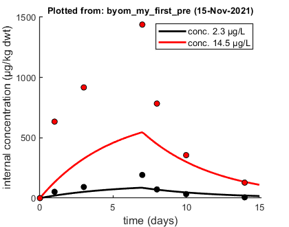
The model runs, and the plot makes sense. The model lines are clearly not optimal fits, but they are close enough for the optimisation routine to do its job. Note the output on screen: BYOM tells you what it did, with which parameters, and what the minus log-likelhood (the optimisation criterion) is at this point.
Then, optimise. Now, let's run the optimisation routine by calling calc_optim (the opt_optim is used for setting optional options, don't worry about them now):
opt_optim.it  = 0; % show iterations of the optimisation (1, default) or not (0)
% Don't show iterations in this demo, as it will fill the page with
% optimisation steps. In general, it is good to leave them on (which is the
% default setting), especially when the model runs are slow.

% optimise and plot (fitted parameters in par_out)
par_out = calc_optim(par,opt_optim); % start the optimisation
Goodness-of-fit measures for each state and each data set (R-square)
Based on the individual replicates, accounting for transformations, and including t=0
state 1.   0.98
=================================================================================
Results of the parameter estimation with BYOM version 6.0 BETA 6
=================================================================================
   Filename      : byom_my_first_pre
   Analysis date : 15-Nov-2021 (16:42)
   Data entered  :
     data state 1: 7x2, continuous data, no transf.
   Search method: Nelder-Mead simplex direct search, 2 rounds.
     The optimisation routine has converged to a solution
     Total 69 simplex iterations used to optimise.
     Minus log-likelihood has reached the value 84.13 (AIC=172.26).
=================================================================================
Kiw         95.99 (fit: 1, initial: 50)
ke         0.4625 (fit: 1, initial: 0.2)
=================================================================================
Time required: 2.0 secs
This is the output report of the optimisation routine; it gives you everything you wanted to know (and probably more). The same output is also saved to a log file (results.out), so you can always look back at older runs (good idea to throw this file away once in a while, as it continues to grow).
The goodness-of-fit measure shown is the r-square, after any transformation have been applied (in this case, we did not transform). The output provides a number of identifiers for your reference, such as BYOM version, file name and date/time. The output shows what type of data you entered, which optimisation was used, and the final minus-log-likelihood achieved (the lower, the better the fit).
Now, the variable par_out contains our optimised parameter set. We can check to make sure:
par_out
par_out =

  struct with fields:

           Kiw: [95.9880 1 0 1000000 1]
            ke: [0.4625 1 1.0000e-03 100 1]
    tag_fitted: 'y'
Note the extra tag that is added to let subsequent routines know that these parameters resulted from an optimisation. You could use these values as the new starting values for another optimisation (in general, that is a good idea, especially for parameter-rich models). You could manually copy the output from screen to your script (in the par structure with initial values), but there is a smarter way, by invoking a little function:
print_par(par_out) % display the contents of par_out in a formatted way
par.Kiw    = [    95.988  1          0      1e+06 1];
par.ke     = [    0.4625  1      0.001        100 1];
Now you can directly use copy-paste to make a new par matrix in your script.
Plot the best fit. Now that we have the optimised parameter set in par_out, we can plot it with the data, by calling the plotting routine calc_and_plot again, but now with the optimised parameter structure par_out:
calc_and_plot(par_out,opt_plot); % calculate model lines and plot them
Plots result from the optimised parameter values.
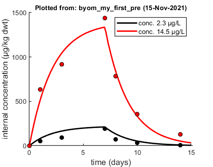
The plot looks nice. By default, BYOM plots in color, using different colors for different scenarios (first row in X0mat). However, there is a plotting option to plot in black and white, using different markers for different scenarios.
Confidence intervals. Every parameter estimate requires a confidence interval. I advise you to use the profile likelihood to construct these intervals. This is a robust method that will not only give you intervals but can also often tell if there is a better optimum to be had elsewhere in parameter space.
To make a profile of parameter Kiw:
calc_proflik(par_out,'Kiw',opt_prof); % calculate and plot the profile likelihood
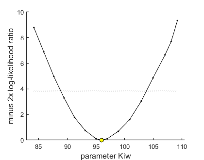
95% confidence interval(s) from the profile(s)
=================================================================================
Kiw        interval:      88.86 -  103.8
=================================================================================

Time required: 5.2 secs
The routine returns the 95% confidence interval for Kiw, which it has calculated from this graph. An explanation will follow in a later chapter, but note that the value of Kiw is plotted on the x-axis. The yellow circle denotes the best value as identified from the optimisation. The black points are new optimisations, fixing Kiw each time to values away from the best fit value. The horizontal line is a cut-off criterion: all values that are below this line are part of the confidence interval.
Statistical and other notes
The analysis above makes sense, but there are a few notes and statistical warnings that I would like to add for completeness:
- It is a bit silly to use an ODE solver to tackle the equation for the one-compartment model given above, as an analytical solution can easily be derived. However, as soon as models become more meaningful, they are rapidly beyon analytical solutions. And, this simple model is a good example to demonstrate how BYOM operates.
- The data points were means of 1-3 replicate measurements. Therefore, I should have added weights in the analysis (the number of individual measurements underlying each data point). However, it would be even better to use the individual measurements themselves. Both are possible in BYOM, but will be explained later.
- The assumption of indepence of the residuals is allright: each measurement results from a new individual as the analysis of body residues is destructive. Normality may also be allright, but constant variance (homoscedasticity) is doubtful. It is likely that small values have less variance than large ones. Therefore, I would suggest a form of transformation on this data set (e.g., log-transformation). This is also possible with BYOM, and explained later.
- The profiling is way more robust than asymptotic standard errors, and relies less stringently on 'asymptotic' theory (i.e., it works well with small data sets). However, the cut-off criterion is based on asymptotic theory, so the intervals will be less reliable with smaller data sets. This is nit-picking, as people generally rely without second thought on the much less reliable 'standard error' and the intervals they yield.
- The likelihood function for the normally-distributed residuals requires an estimate of the residual variance (which we don't know). This variance is treated as a nuisance parameter, and profiled out. The different treatments within a data set are assumed to share the same residual variance, but different data sets have their own variance. This generally works well, but given sufficient interest I will be tempted to include more refined options. Note that BYOM also allows you to supply a residual variance per data set.
- The optimisation routine is a Nelder-Mead simplex search (fminsearch in Matlab). Two runs are performed in sequence, the first with a low number of maximum iterations, which passes its optimised parameters to a second (default setting) one. I found this to be a useful enough strategy to implement as default.
- BYOM offers a lot of options to modify its functions. You saw them in the Matlab calls above as opt_optim, opt_plot and opt_prof. These options are structures that are filled automatically by the BYOM script. So, you only overwrite options if you like to depart from default behaviour. All options are described in a text file all_options.txt in the BYOM folder.
- BYOM offers several other approaches for making confidence intervals and plotting results. E.g., there is a possibility to obtain a Bayesian sample from the posterior distribution, and create intervals on model curves. These will be treated later.
Continu to next step
Next: byom_my_first.m to walk through this analysis in a formal way (Matlab-published version of the full script in a BYOM setting).