SIMbyom, byom_sim_rosmac.m, Rosenzweig-MacArthur model
- Author: Tjalling Jager
- Date: November 2021
- Web support: http://www.debtox.info/byom.html
- Back to index walkthrough_simbyom.html
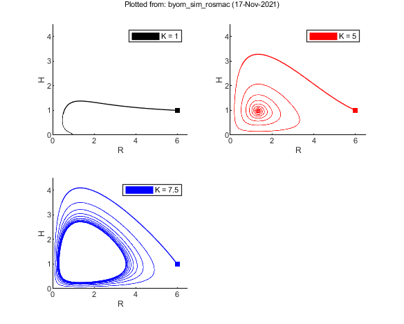
This is the classical Rosenzweig-MacArthur model. More background in http://www.jstor.org/stable/2458702. With low K, the predator (H) goes extinct, with medium K, there is a stable equilibrium, with high K, there is a limit cycle.
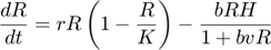
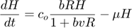
Model system:
Copyright (c) 2012-2021, Tjalling Jager, all rights reserved.
This source code is licensed under the MIT-style license found in the
LICENSE.txt file in the root directory of BYOM.
Contents
Initial things
Make sure that this script is in a directory somewhere below the BYOM folder.
clear, clear global % clear the workspace and globals
global glo X0mat    % allow for global parameters in structure glo
diary off           % turn of the diary function (if it is accidentaly on)
% set(0,'DefaultFigureWindowStyle','docked'); % collect all figure into one window with tab controls
set(0,'DefaultFigureWindowStyle','normal'); % separate figure windows

pathdefine % set path to the BYOM/engine directory
glo.basenm  = mfilename; % remember the filename for THIS file for the plots
Initial values for the state variables
Initial states, scenarios in columns, states in rows. First row are the 'names' of all scenarios.
% Initial states, first row is different values for K
X0mat(1,:) = [1 5 7.5];
X0mat(2,:) = 6;
X0mat(3,:) = 1;
Values for the model parameters
Model parameters are part of a 'structure' for easy reference.
% syntax: par.name = value
par.r   = 1;    % growth rate of resource
% par.K   = 7.5;  % carrying capacity of resource (scenario name is now used)
par.b   = 1;    % searching rate of consumer
par.v   = 0.25; % handling time of consumer
par.co  = 1;    % conversion factor resource to consumer
par.mu  = 1;    % maintenance rate for consumer
Time vector and labels for plots
Specify what to plot. If time vector glo.t is not specified, a default is used, based on the data set
glo.t = linspace(0,100,5000); % time vector for the model curves

% specify the y-axis labels for each state variable
glo.ylab{1} = 'R';
glo.ylab{2} = 'H';
% specify the x-axis label (same for all states)
glo.xlab    = 'time';

glo.leglab1 = 'K = '; % legend label before the 'scenario' number
glo.leglab2 = ''; % legend label after the 'scenario' number

% If needed, a stiff solver or events function can be selected in call_deri
Optional settings for the simulations
opt_sim.plot_int = 100; % interval for plotting (how many time points to do in one go), default: 10
opt_sim.axrange  = [0 6.5;0 4.5]; % axis ranges for states, default: autoscale

opt_sim.plottype = 6; % default: 4
% 1) 3d plot
% 2) 2d plot
% 3) states in subplots
% 4) scenarios in subplots
% 5) dx/dt versus x
% 6) 2d plot for each scenario separate
% 7) 3d plot for each scenario separate
Calculations and plotting
Here, the script is called that will do the calculation and the plotting. The squares in the graph indicate the starting points. In the top of the file sim_and_plot.m, there are several more options to modify the plotting.
sim_and_plot(par,opt_sim); % call the script which calculates and plots