SIMbyom, byom_sim_lorenz.m, the Lorenz attractor
- Author: Tjalling Jager
- Date: November 2021
- Web support: http://www.debtox.info/byom.html
- Back to index walkthrough_simbyom.html
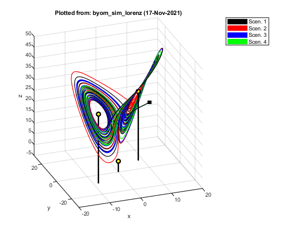
This is the classical Lorenz system. Default parameter set leads to a chaotic solution. Background: https://en.wikipedia.org/wiki/Lorenz_system
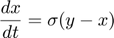
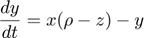
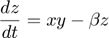
Model system:
Copyright (c) 2012-2021, Tjalling Jager, all rights reserved.
This source code is licensed under the MIT-style license found in the
LICENSE.txt file in the root directory of BYOM.
Contents
Initial things
Make sure that this script is in a directory somewhere below the BYOM folder.
clear, clear global % clear the workspace and globals
global glo X0mat    % allow for global parameters in structure glo
diary off           % turn of the diary function (if it is accidentaly on)
% set(0,'DefaultFigureWindowStyle','docked'); % collect all figure into one window with tab controls
set(0,'DefaultFigureWindowStyle','normal'); % separate figure windows

pathdefine % set path to the BYOM/engine directory
glo.basenm  = mfilename; % remember the filename for THIS file for the plots
Initial values for the state variables
Initial states, scenarios in columns, states in rows. First row are the 'names' of all scenarios. Note that we here have a situation where the 4 starting points are very close together, only differing slightly in their x-value.
% scenarios specify different starting conditions, for rho = 28
X0mat(1,:) = [1 2 3 4];
X0mat(2,:) = [10 10.1 10.2 10.3];
X0mat(3,:) = 0;
X0mat(4,:) = 25;
Values for the model parameters
Model parameters are part of a 'structure' for easy reference.
% syntax: par.name = value
par.sig   = 10;  % sigma
par.rho   = 28;  % rho
par.bet   = 8/3; % beta
Time vector and labels for plots
Specify what to plot. If time vector glo.t is not specified, a default is used, based on the data set
glo.t = linspace(0,20,10000); % time vector for the model curves

glo.ylab{1} = 'x';
glo.ylab{2} = 'y';
glo.ylab{3} = 'z';
% specify the x-axis label (same for all states)
glo.xlab    = 'time';

glo.leglab1 = 'Scen. '; % legend label before the 'scenario' number
glo.leglab2 = ''; % legend label after the 'scenario' number

% If needed, a stiff solver or events function can be selected in call_deri
Optional settings for the simulations
opt_sim.plot_int = 50; % interval for plotting (how many time points to do in one go), default: 10
opt_sim.axrange  = [-20 20; -30 30; -5 50]; % axis ranges for each state, default: autoscale

opt_sim.plottype = 1; % default: 4
% 1) 3d plot
% 2) 2d plot
% 3) states in subplots
% 4) scenarios in subplots
% 5) dx/dt versus x
% 6) 2d plot for each scenario separate
% 7) 3d plot for each scenario separate

% which states to plot on which axes? For 2d and 3d plots. Default: x=1, y=2, z=3
opt_sim.stxyz = [1 2 3]; % state number for x-, y- and z-axis

% equilibrium points (comment out if not known)
opt_sim.Xeq(1,:) = [sqrt(par.bet*(par.rho-1));sqrt(par.bet*(par.rho-1));par.rho-1];
opt_sim.Xeq(2,:) = [-sqrt(par.bet*(par.rho-1));-sqrt(par.bet*(par.rho-1));par.rho-1];
opt_sim.Xeq(3,:) = [0;0;0];

% X0mat = [1 2 3; Xeq'+0.1]; % start close to the equilibria
Calculations and plotting
Here, the script is called that will do the calculation and the plotting. The yellow points in the graph indicate the equilibrium points, and the squares the starting points. In the top of the file sim_and_plot.m, there are several more options to modify the plotting.
sim_and_plot(par,opt_sim); % call the script which calculates and plots